DKX
dkx solves the radially local, linearized drift-kinetic equation on a
flux surface — the same physics as SFINCS Fortran v3 — in pure JAX. One
input.namelist plus one geometry file gives neoclassical particle/heat
fluxes, parallel flows, bootstrap current, and transport matrices for
stellarators and tokamaks, on CPU or GPU, with end-to-end automatic
differentiation for sensitivities and optimization.
Quickstart
pip install dkx
from pathlib import Path
from dkx.run import run_profile

run = run_profile(Path("input.namelist"), solve_method="auto",
                  out_path=Path("sfincsOutput.h5"))
print(float(run.moments["particleFlux_vm_psiHat"][0]))
print(float(run.moments["FSABjHat"]))  # bootstrap current <j.B>
run_profile prints the Fortran-parity console flow, writes
sfincsOutput.h5/.nc keyed by the SFINCS output names, and returns the
state vector, solver statistics, and all velocity-space moments in memory. The
CLI equivalent is dkx input.namelist --out sfincsOutput.h5;
dkx --plot sfincsOutput.h5 builds a PDF diagnostics panel. See
Installation for the solvax structured-solver core dependency, GPU
wheels, and the Fortran reference build.
Examples
Six pedagogic scripts on the canonical API sit at the top of examples/
(no main(), parameters at the top, printed progress, a plot, outputs
written and read back); Examples walks through each one:
examples/getting_started/run_tokamak.py— build a namelist in Python, solve a circular tokamak, read HDF5/NetCDF back.examples/getting_started/run_w7x.py— W7-X Boozer geometry with full Fokker-Planck collisions (tier-2 recycled Krylov).examples/transport/transport_coefficients.py— monoenergetic transport matrices and a collisionality scan.examples/vmex_finite_beta/ambipolar_er_scan.py— scan the radial electric field and solve the ambipolar root.examples/autodiff/gradients_tour.py—jax.gradthrough the kinetic solve, verified against finite differences.examples/optimization/optimize_QA_bootstrap.py— flagship gradient-based QA stellarator optimization with kinetic<j.B>in the objective.
Performance and parity evidence
Performance and differentiability records the measured canonical-stack evidence: on the
744k-unknown HSX PAS/DKES case, the tier-1 structured solve completes in
27.2 s at 0.93 GB on a MacBook M4, versus 463.6 s / 3.98 GB
for 1-rank SFINCS Fortran v3 and 229.5 s / 2.86 GB at its measured
2-rank parallel floor. Parity referees pin RHSMode=1 output tables to
8e-14, state vectors to 1e-11, and transport matrices to
6e-13 .. 9e-9 against Fortran golden data.
A broader example-suite benchmark complements that single case: it runs the
full 39-case CPU/GPU example suite against SFINCS Fortran v3 and plots every
row whose Fortran reference runtime clears a 10 s reference-runtime-window,
so process-launch and JIT-amortization noise does not dominate the bars.
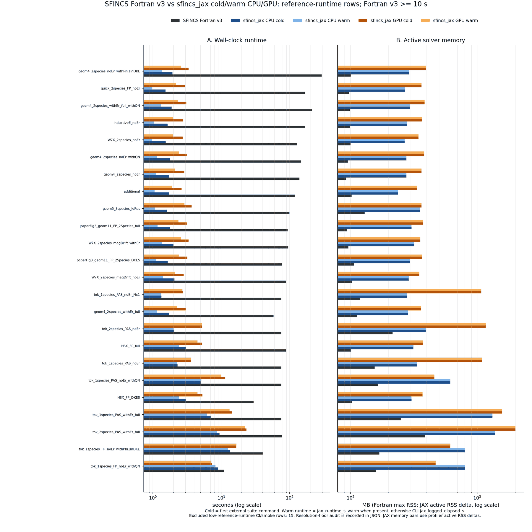
Example-suite benchmark for rows whose SFINCS Fortran v3 reference runtime is
at least 10 s. Fortran memory is process maximum RSS; JAX memory uses
profiler RSS deltas over the fixed runtime baseline. Reproduce with
examples/publication_figures/generate_fortran_suite_benchmark_summary.py.
What this documentation covers
getting started: Installation, Usage, Examples
physics and numerics: Physics model and equations, Drift-kinetic equation and system of equations, Geometry models and loading, Method overview, Numerics and algorithms, Differentiability, Reduced-model capabilities
references: Inputs (namelist) reference, Outputs (HDF5, NetCDF4, and NPZ), Normalizations and units, Source-code map, API reference
evidence: Performance and differentiability, Parity status, Fortran v3 And dkx Feature Matrix, Validation against reference implementations, Validation Matrix
workflows: Applications and research workflows, Optimization Workflows, Parallelism, VMEC JAX workflow
Contents
- Installation
- Applications and research workflows
- Optimization Workflows
- Examples
- Canonical examples
- Example tree
- One-command start points
- Decision map
- Application recipe map
- Top-level folder categories
- Finite-beta VMEX to kinetic transport
- Transport matrices (RHSMode=2/3)
- Upstream postprocessing (utils/)
- Optimization + figures
- Implicit differentiation through solves
- VMEC-to-Boozer Differentiable Geometry Workflow
- Parallel and scaling examples
- Upstream SFINCS example inputs
- Usage
- Parsing an input file
- Building v3 grids and geometry
- Supported geometry examples
- Applying the operator directly
- Running the Fortran v3 executable
- First CLI run
- Advanced linear-state export
- Advanced solver controls
- Parallel CLI controls
- Environment variables
- Writing output files with dkx
- Running an
Erscan (transport-matrix mode) - Solving the ambipolar root directly
- Running upstream postprocessing scripts (utils/)
- Inputs (namelist) reference
- Outputs (HDF5, NetCDF4, and NPZ)
- Normalizations and units
- Geometry models and loading
- VMEC JAX workflow
- Method overview
- Numerics and algorithms
- Differentiability
- Reduced-model capabilities
- Source-code map
- Fortran v3 And dkx Feature Matrix
- Theory from the upstream SFINCS notes
- Ordering and reduction used by SFINCS v3
- Normalization hierarchy
- Drives, fluxes, and transport-matrix columns
- Constraint structure and nullspaces
- Monoenergetic and DKES-like limits
- Fokker-Planck field terms and Rosenbluth potentials
- Phi1, quasineutrality, and poloidally varying collisions
- What this means for dkx engineering
- Primary sources summarized here
- Physics model and equations
- Physics reference: the radially local drift-kinetic model
- Governing equation and the \(f_0+f_1\) split
- Normalization: \(\Delta\), \(\alpha\), \(\nu_n\)
- Streaming and mirror terms
- \(E\times B\) drift
- Radial-electric-field energy and pitch-angle drifts
- Thermodynamic and inductive drives
- Collision operators
- Flux-surface potential variation \(\Phi_1\) and quasineutrality
- Moments, fluxes, and transport coefficients
- Ambipolarity and the radial electric field
- Classical (collisional) transport
- Equation-to-code map
- Upstream derivations
- Drift-kinetic equation and system of equations
- Parallelism
- Open research lanes
- Performance and differentiability
- Development Roadmap
- Speed grids (canonical) and the retired adaptive-map research lane
- Testing, validation, and CI
- Validation Matrix
- Paper figures (reproduced)
- Upstream SFINCS sources and primary literature
- Fortran v3 example suite status
- Utils (ported SFINCS v3 scripts)
- API reference
- Validation against reference implementations
- References and related work
- Foundational neoclassical theory
- SFINCS model, collision operator, and speed grid
- Block-tridiagonal Legendre solver and variational bounds
- Geometry and benchmark configurations
- Experimental and cross-code validation anchors
- Upstream SFINCS technical notes and manuals
- JAX and differentiable programming
- Testing, validation, and coverage methodology
- Linear algebra and preconditioning
- Optimization-focused neoclassical workflows
- Recent applications (examples to prioritize)
- Contributing
- Release notes
- Release checklist