Differentiability
dkx is differentiable end to end. Because the drift-kinetic operator,
its right-hand side, and the moment diagnostics are all pure JAX functions, a
scalar built from a solved distribution — a flux, a bootstrap current, an
ambipolar \(E_r\), a transport coefficient — can be handed straight to
jax.grad and returns an exact derivative with respect to geometry harmonics,
plasma profiles, or the collisionality. There is no divided-difference
stencil in the loop and no differentiation through solver iterations.
This page explains how the gradient is taken through the linear solve, catalogues
what is differentiable, reports the measured gradient-vs-finite-difference
agreement, and shows the differentiable geometry chain
vmex -> booz_xform_jax -> dkx used for stellarator optimization.
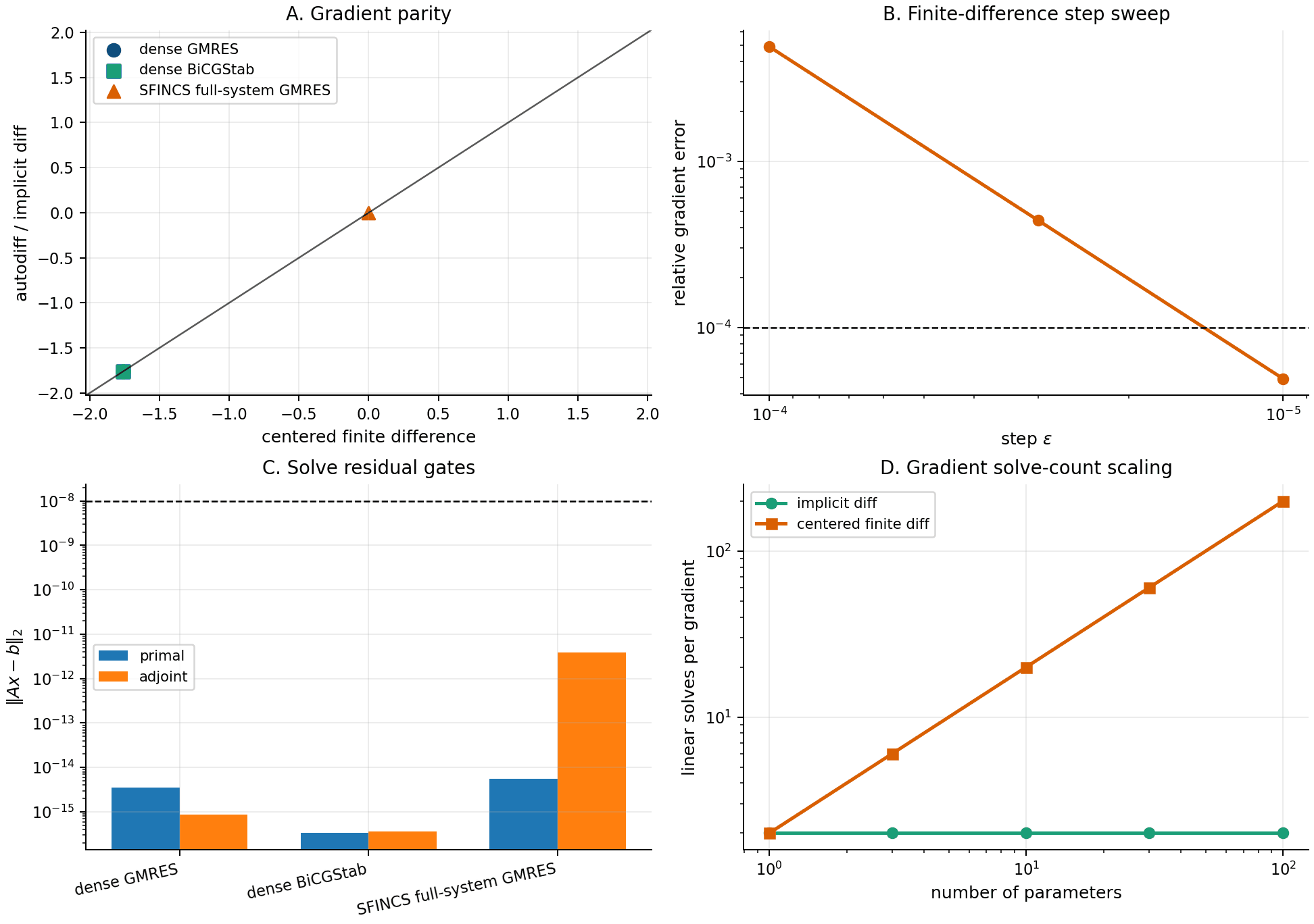
Reverse-mode jax.grad derivatives of kinetic observables (points) plotted
against centered finite differences (line). Reproduce with
examples/autodiff/gradients_tour.py.
Implicit differentiation through the solve
Every tier of the solver returns the solution of a linear system \(A(p)\,u = b(p)\), where \(p\) collects the differentiable parameters (geometry, profiles, drives). For a scalar objective \(J = g(u, p)\) the chain rule needs \(\mathrm{d}u/\mathrm{d}p\), which satisfies the tangent system
Differentiating through the Krylov or block-elimination iterations to get this would be expensive and numerically noisy. Instead the solve is wrapped with the implicit function theorem: the reverse-mode adjoint of \(A u = b\) is the single transposed solve
The decisive point is that \(A^{\mathsf T}\lambda = \cdot\) reuses the
forward factorization. In tier 1 the adjoint is the same block-Thomas sweep run
with transpose=True on the factors already computed for the forward solve; in
tier 2 it is the transposed-preconditioner recycled-Krylov solve seeded from the
same coarse operator. A gradient therefore costs one extra solve, independent
of how many iterations the forward solve took.
The wrappers come from the standalone solvax package: linear solves route
through solvax.implicit.linear_solve (jax.lax.custom_linear_solve), and
the outer root problems — the ambipolar \(E_r\) and the nonlinear
\(\Phi_1\) Newton solve — route through solvax.implicit.root_solve
(jax.lax.custom_root), so their derivatives also fall out of the implicit
function theorem rather than unrolled iterations.
Where in the code
solve(op, rhs, differentiable=True) (dkx.solve.solve()) wraps
tiers 1 and 2 with the implicit adjoint. The scalar
ambipolar_er (dkx.er.ambipolar_er()) and the
phi1_state (dkx.phi1.phi1_state()) helpers return
differentiable JAX arrays directly. The tier-3 host direct solve is not
differentiable and raises if differentiable=True is requested.
What is differentiable
Target |
What flows |
Entry point |
|---|---|---|
Geometry |
Boozer harmonics \(\hat B_{mn}\) and derived metric coefficients, for analytic schemes and for JAX-native geometry producers |
|
Profiles |
densities, temperatures, their radial gradients, |
|
Ambipolar \(E_r\) |
the scalar root of \(J_r(E_r)=0\) and any downstream function of it |
|
\(\Phi_1\) state |
the solved flux-surface potential \(\Phi_1(\theta,\zeta)\) from the nonlinear quasineutrality Newton solve |
|
Monoenergetic transport matrix |
the RHSMode=3 coefficients and the energy-convolved thermal \(L_{ij}\), differentiated w.r.t. geometry |
|
The file-based readers (input.namelist, .bc Boozer files, wout_*.nc)
are provenance and parity tools and are not differentiable. Geometry
sensitivities flow through JAX-native producers instead — the analytic geometry
schemes, or the vmex -> booz_xform_jax transform below.
Note
The differentiable ambipolar \(E_r\) and \(\Phi_1\) helpers require the
untruncated pitch embedding (Nxi_for_x_option = 0); with an active
\(N_\xi\)-for-\(x\) ramp they raise NotImplementedError rather than
return an approximate gradient. RHSMode=1 outputs remain differentiable through
the ramped tier-1 route.
Measured gradient accuracy
Every differentiable path is gated against centered finite differences. The recorded agreements are:
Differentiable target |
Adjoint route |
|
|---|---|---|
PAS + \(E_r\) kinetic outputs |
tier-2 recycled-Krylov transposed solve |
|
Ramped-PAS RHSMode=1 output |
tier-1 truncated block-Thomas, transposed |
agree at rtol |
Monoenergetic \(L_{11}\) w.r.t. \(\hat B_{mn}\) |
tier-1 differentiable + energy convolution |
|
Monoenergetic energy convolution to thermal \(L_{ij}\) |
closed-form convolution vs a full RHSMode=2 kinetic solve |
|
As a throughput reference, a value_and_grad of a 39,318-unknown PAS
scheme-1 objective through the tier-1 differentiable route costs about
5.3 s cold and 2.1 s warm on the development MacBook — the adjoint adds
roughly one forward solve, as predicted.
Warning
Do not trust a tier-2 gradient on a numerically singular Fokker-Planck
system. Full Fokker-Planck with constraintScheme=1 on the flagship
optimization deck produces a near-singular operator (about 5 zero singular
values, condition number \(\sim 2\times10^{36}\)). The recycled-Krylov
adjoint stagnates and the vector-Jacobian product returns a wrong gradient
with no error raised (-1.7e-3 from autodiff versus +2.8e-5 from finite
differences on the affected degree of freedom). The PAS + \(E_r\) gradient
on the same optimization chain is exact. Until the adjoint residual is
surfaced in SolveResult and flagged when it misses tolerance, validate
gradients on singular-FP decks against a finite difference before using them.
The differentiable optimization chain
Stellarator optimization with a kinetic objective closes the loop from the plasma boundary to a neoclassical figure of merit and back, entirely under automatic differentiation:
Each arrow is a JAX transformation, so jax.grad of the bootstrap current
\(\langle \mathbf{j}\cdot\mathbf{B}\rangle\) (or a transport coefficient)
with respect to the boundary Fourier modes propagates through the equilibrium
solve, the Boozer transform, and the drift-kinetic solve without any finite
differences. The flagship script examples/optimization/optimize_QA_bootstrap.py drives a
quasi-axisymmetric, low-bootstrap optimization on exactly this chain with warm
starts and finite-difference-verified gradients; the geometry link on its own is
demonstrated in examples/autodiff/vmex_to_boozer_sfincs_pipeline.py. See
Optimization Workflows and VMEC JAX workflow for the full workflow.
Worked examples
examples/autodiff/gradients_tour.py—jax.gradof kinetic outputs through the implicit solve, checked against finite differences (the figure above).examples/autodiff/matrix_free_residual_and_jvp.py— matrix-free residual and Jacobian-vector products for the F-block.examples/autodiff/implicit_diff_through_gmres_solve_scheme5.py— implicit differentiation through a full-system Krylov solve on a VMEC geometry.examples/autodiff/differentiable_geometry_gradients.py— a geometry scalar differentiated with respect to harmonic amplitudes.examples/optimization/optimize_QA_bootstrap.py— the flagship gradient-based optimization with kinetic \(\langle \mathbf{j}\cdot\mathbf{B}\rangle\) in the objective.
See Numerics and algorithms for the solver tiers behind the adjoint and Performance and differentiability for runtime and memory of the differentiable paths.