Paper figures (reproduced)
This page collects reproducible validation figures generated by running the corresponding dkx cases. Figures 1 and 2 are backed by audited full-resolution JSON summaries; fast variants remain available in the publication-figure scripts for branch-level regression checks.
Generate the SFINCS-paper reproduction figures with
python examples/publication_figures/generate_sfincs_paper_figs.py --fast
Omit --fast to use the default scan resolution.
Generate the publication validation dashboard with
python examples/publication_figures/generate_validation_dashboard.py
Generate the frozen CPU/GPU Fortran-suite runtime and memory comparison with
python examples/publication_figures/generate_fortran_suite_benchmark_summary.py
The default figure filters to reference-runtime-window rows whose Fortran v3
runtime is at least 10 s. The summary JSON records which frozen rows are
excluded from public performance claims until matching production-resolution
reruns exist. Use --min-fortran-runtime-s 0 only for all-case CI/smoke
diagnostics, not for public performance claims.
Generate the autodiff/sensitivity validation figures with
python examples/publication_figures/generate_autodiff_sensitivity_validation.py
Dashboard
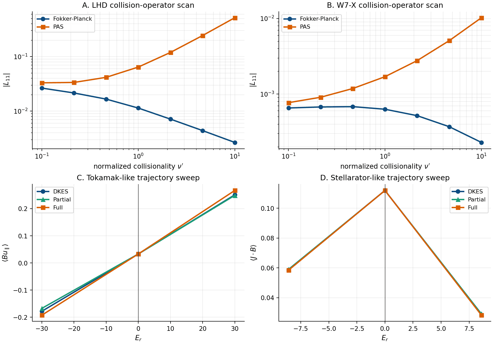
Publication dashboard generated from checked-in JSON artifacts. Panels A-B show
the LHD and W7-X collision-operator collisionality scans used to audit FP/PAS
behavior in the SFINCS 2014 validation setting. Panels C-D show the pinned
trajectory-model sweeps used to verify exact zero-field agreement and finite-field
separation between DKES, partial, and full trajectory models. The machine-readable
summary is
examples/publication_figures/artifacts/dkx_publication_validation_dashboard_summary.json.
Fortran v3 suite benchmark
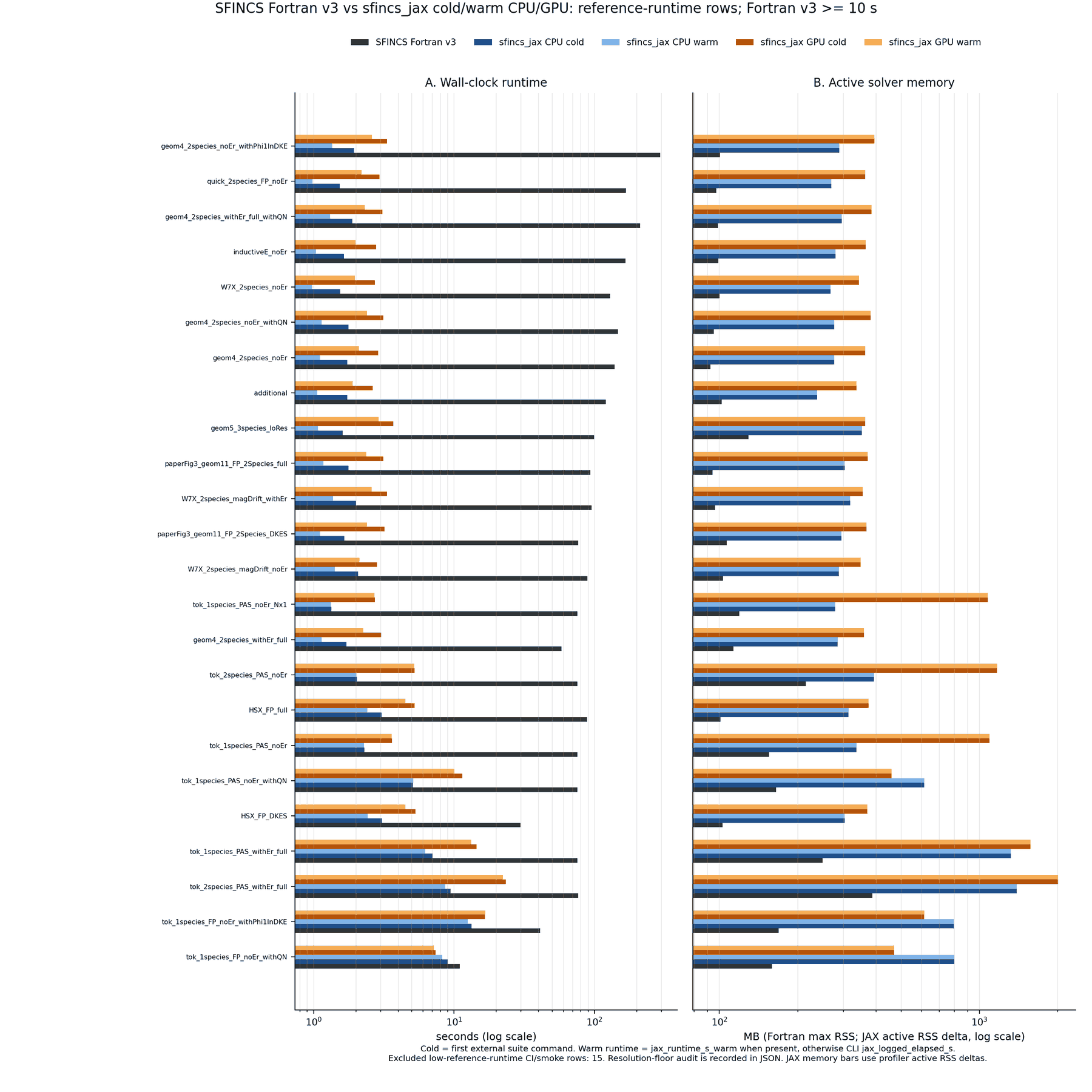
Runtime and memory comparison generated from the frozen full-suite reports.
Panel A shows wall-clock runtime and Panel B shows active solver memory for
SFINCS Fortran v3, dkx CPU cold/warm, and dkx GPU
cold/warm across the reference-runtime-window subset. Both panels use log-scaled axes.
Fortran memory is process maximum RSS; JAX memory uses profiler RSS deltas
over the fixed Python/JAX/XLA baseline, with full process RSS retained in the
JSON audit fields.
Cases are ordered by best warm dkx speedup over the Fortran v3
runtime, placing the strongest JAX wins first.
Cold is the first external suite command. Warm runtime uses
jax_runtime_s_warm when rerun timings are present and otherwise uses the
recorded jax_logged_elapsed_s fallback; the JSON summary records
warm_or_logged_runtime_source_counts. The machine-readable summary,
including parity status, runtime/memory ratios, and the excluded sub-10 s
Fortran rows, is
examples/publication_figures/artifacts/dkx_fortran_suite_benchmark_summary.json.
Autodiff and sensitivity validation
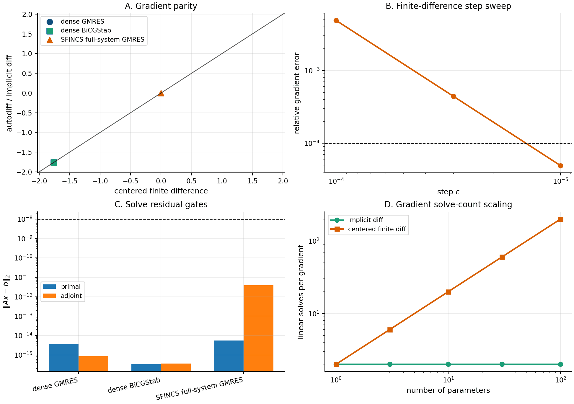
Gradient-validation dashboard for the differentiable solve path. Panel A compares
autodiff/implicit-diff gradients with centered finite differences for stable scalar
objectives, including a pinned SFINCS full-system linear solve. Panel B records the
finite-difference step sweep used for the SFINCS gradient gate. Panel C shows primal
and adjoint residuals for the solve checks. Panel D shows the solve-count advantage
of implicit differentiation over centered finite differences as the number of
parameters grows. The machine-readable summary is
examples/publication_figures/artifacts/dkx_autodiff_sensitivity_validation_summary.json.
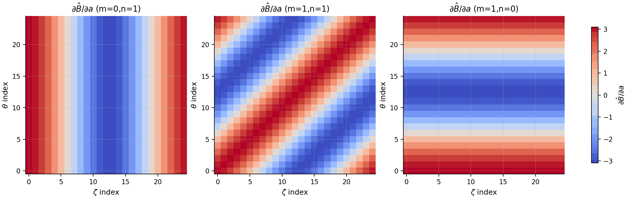
Spatial sensitivity maps for the differentiable geometryScheme=4 Boozer
harmonic amplitudes. This is a bounded manuscript artifact: it validates the JAX
sensitivity machinery for the public analytic-Boozer geometry path, while full
VMEC-boundary optimization remains a separate research workflow.
High-collisionality trend proxy
The checked trend proxy is retained as compact JSON and figure evidence. The long generator lives on the publication-audits research branch; stable docs use the checked artifact and package-level validation tests.
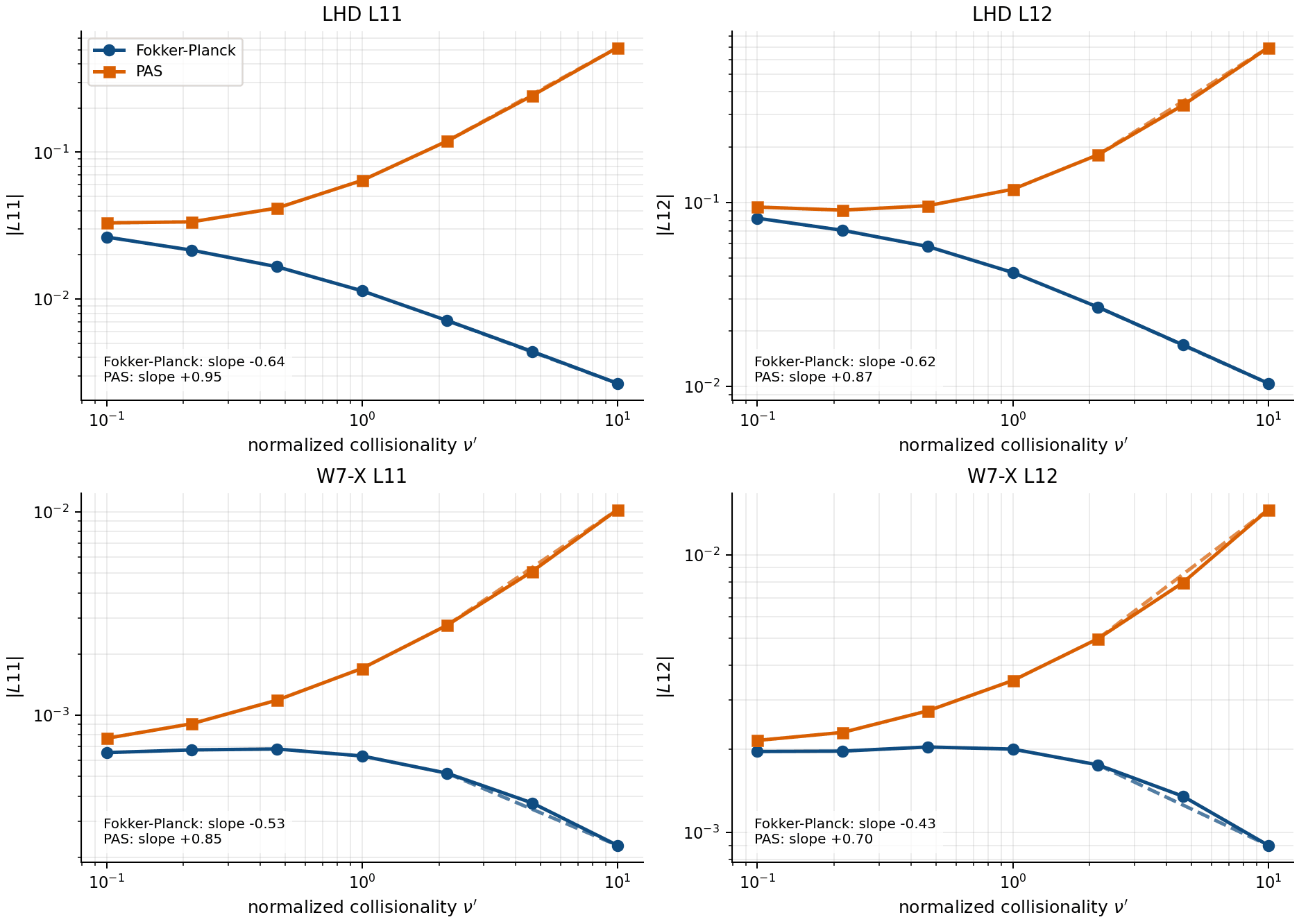
Power-law tail fits for L11 and L12 from the corrected full LHD and W7-X
collisionality artifacts. This is a trend proxy, not the final
Simakov-Helander analytic-limit reproduction: the LHD Fokker-Planck tail passes
the loose inverse-nu trend proxy on the checked-in range, while the W7-X
Fokker-Planck tail still needs a wider nu' >> 1 scan before it can support the
analytic-limit claim. The stricter Simakov-Helander audit below keeps both
geometries deferred until the wider high-nu scan is pinned.
Simakov-Helander limit audit
The normalization/readiness audit is retained as compact JSON and figure evidence. The long audit and high-nu run-plan generators live on the publication-audits research branch.
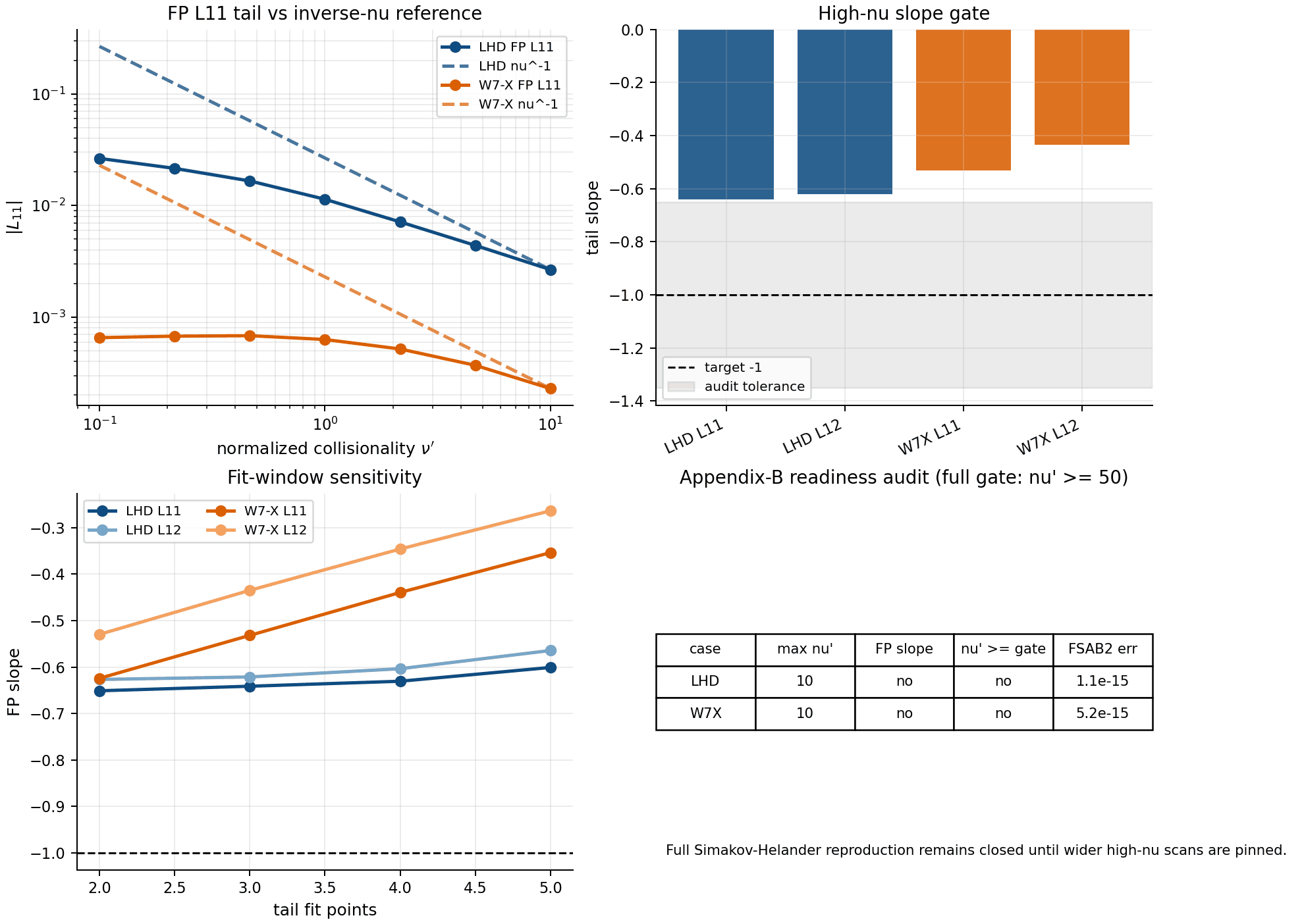
Reviewer-facing audit for the full high-collisionality analytic-limit lane.
The JSON artifact records the Appendix-B geometry ingredients available in
checked-in sfincsOutput.h5 files, recomputes FSABHat2 from BHat and
DHat, tracks the L11/L12 inverse-nu slope proxy, and explicitly
keeps the full Simakov-Helander reproduction closed until wider high-nu
scans are pinned. The machine-readable summary is
examples/publication_figures/artifacts/dkx_simakov_helander_limit_audit_summary.json.
The paired high-nu' run plan is
examples/publication_figures/artifacts/dkx_simakov_helander_high_nu_run_plan.json.
Launch the bounded pilot first so the terminal ETA and residual behavior are visible before committing to the full FP/PAS LHD+W7-X extension:
CUDA_VISIBLE_DEVICES=0,1 \
python examples/publication_figures/generate_sfincs_paper_figs.py \
  --case lhd \
  --collision-operators 0 \
  --nuprime-min 17.78279101649707 \
  --nuprime-max 17.78279101649707 \
  --n-points 1 \
  --timeout-s 900 \
  --transport-workers 2 \
  --transport-parallel-backend gpu \
  --transport-sparse-direct-max 30000 \
  --require-residuals \
  --max-transport-residual 1e-6 \
  --max-transport-relative-residual 1e-6 \
  --skip-existing \
  --scan-only
These executable scans run on the explicit (non-differentiable) performance
path: the scan subprocesses go through the sfincsScan CLI flow, whose
solves are explicit by default — implicit differentiation is opt-in from the
Python API — and the launcher records implicit_solve: false in each run
plan for provenance. The run plan caps sparse direct solves at 30000 active
unknowns by default: the LHD FP pilot remains on the accurate host sparse-LU
path, while larger W7-X FP high-nu' runs must explicitly opt into the
40000 cap after a bounded pilot proves the residual gate is clean. The same
residual thresholds are also used as fail-fast aborts for sequential and
GPU-worker runs, so a bad high-nu' point does not waste the rest of a
campaign once the first failed RHS is known. GPU runs can still opt into larger
host sparse-LU first attempts/rescues when a bounded pilot shows they are useful,
instead of the differentiable implicit path that intentionally avoids host-only
direct solvers.
The two-GPU office pilot for the first LHD FP high-nu' point produced
residuals 4.33e-16, 5.33e-14, and 4.06e-11 in about 262 s. The
same explicit point on one GPU took about 345 s; the implicit-path
comparison took about 569 s and stalled at much larger residuals. The first
full-resolution W7-X FP high-nu' point has a residual-clean route: with one GPU worker,
a float32 sparse-direct factorization, and
--transport-sparse-direct-max 40000, the three RHS residual/RHS/relative
tuples were 1.297471e-10 / 1.885192e-04 / 6.882435e-07,
1.975724e-12 / 2.623896e-04 / 7.529734e-09, and
4.841651e-09 / 6.589011e-01 / 7.348069e-09. With sparse-helper factor
reuse, the scan took about 582 s on one office GPU instead of about
2028 s before reuse; RHS timings were about 574.0 s, 2.47 s, and
2.38 s. The smaller 30000 cap and Krylov-only
preconditioners still fail this point, so the strict residual gates remain
mandatory for widened scans.
W7-X high-nu preconditioning/performance
Generate the W7-X high-nu' performance figure with
python examples/publication_figures/generate_w7x_high_nu_performance.py
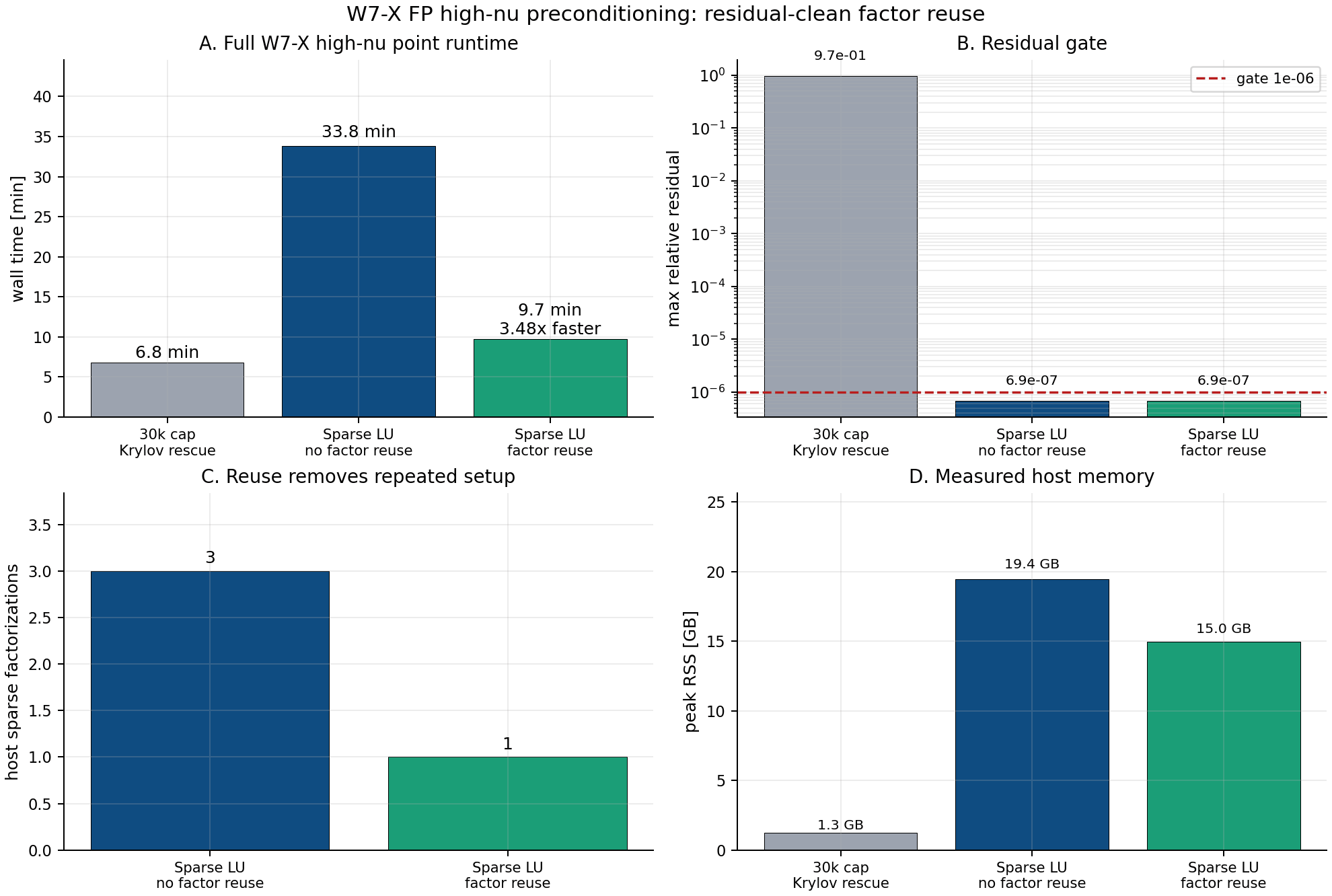
Runtime, residual, setup-count, and peak-RSS comparison for the first
full-resolution W7-X FP high-nu' point. The bounded 30000 cap is
shown as a rejected route because it fails the residual gate. The
factor-reuse sparse-LU route preserves the residual-clean transport matrix
exactly while reducing wall time from about 33.8 min to 9.7 min and
measured peak RSS from about 19.9 GB to 15.3 GB. The machine-readable
summary is
examples/publication_figures/artifacts/dkx_w7x_high_nu_performance_summary.json.
Figure 1 (LHD collisionality scan)
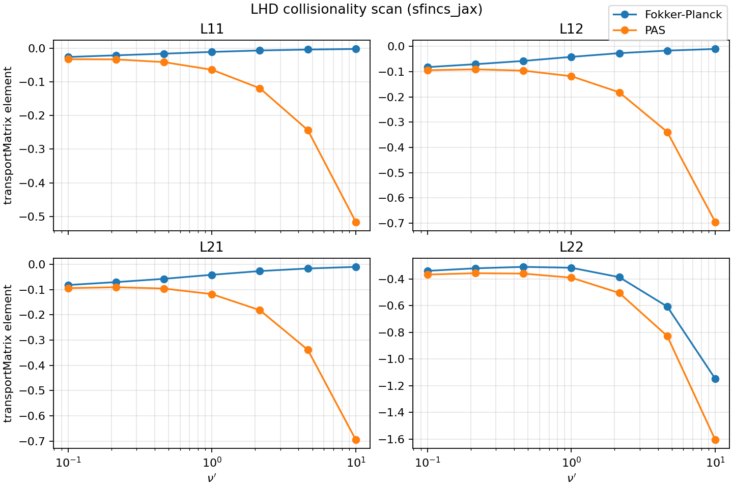
Ion transport matrix elements vs collisionality for LHD geometry at E_r = 0.
Figure 2 (W7-X collisionality scan)
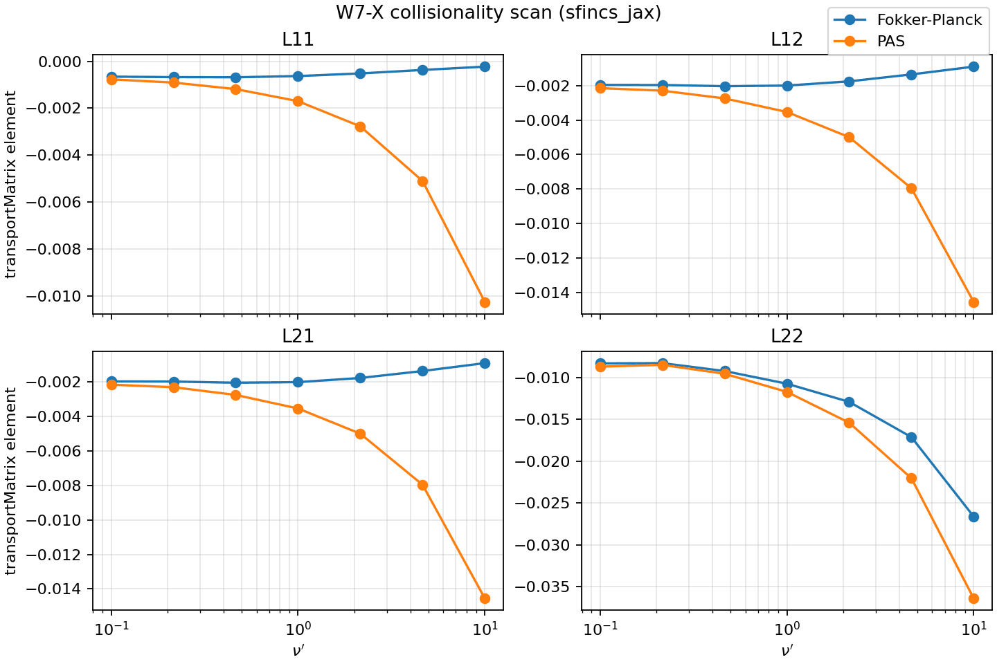
Ion transport matrix elements vs collisionality for W7-X geometry at E_r = 0.
Figure 3 (Simakov–Helander limits)
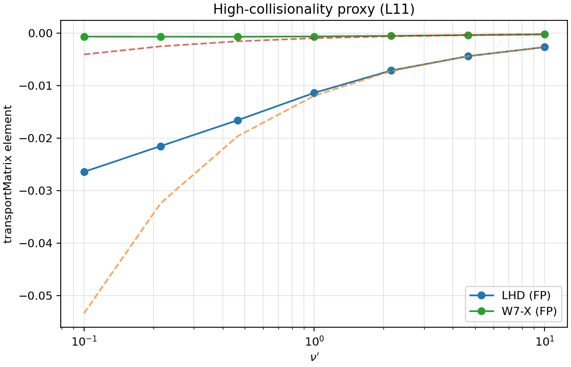
Historical high-collisionality proxy from the SFINCS-paper figure generator. Use
the normalization/readiness audit above for reviewer-facing claims until a wider
high-nu Simakov-Helander reproduction is generated from pinned scan outputs.