Examples

Canonical examples

Six pedagogic scripts on the canonical API sit at the top of examples/. Each follows the same style contract: no main(), all parameters at the top of the file, printed setup/progress/final results, at least one plot, and output files written and read back. All run on a laptop CPU; CI runs each one at shrunken resolution (DKX_CI=1) in tests/test_examples_pedagogic.py.

examples/getting_started/run_tokamak.py — first solve, from Python

Builds a circular-tokamak input.namelist from Python dicts (geometryScheme=1, one ion species, pitch-angle-scattering collisions), runs the canonical driver, and reads the HDF5 output back. The key lines:

from dkx.run import run_profile

run = run_profile(deck_path, solve_method="auto", out_path=h5_path)
gamma = float(run.moments["particleFlux_vm_psiHat"][0])

It teaches the per-species results table, the four radial-coordinate flux conventions, and HDF5/NetCDF output selection by file suffix.

examples/getting_started/run_w7x.py — stellarator geometry and full Fokker-Planck

Loads a W7-X Boozer equilibrium and solves with the linearized Fokker-Planck operator, which routes auto to the tier-2 recycled-Krylov (GCROT) solver instead of the tier-1 structured direct path. It teaches geometry files, collision-operator selection, and how to inspect which solver tier ran (run.solve_result.method).

examples/transport/transport_coefficients.py — RHSMode=3 transport matrices

Computes monoenergetic transport matrices over a collisionality scan, checks Onsager symmetry, and plots L11 versus nuPrime.

examples/vmex_finite_beta/ambipolar_er_scan.py — ambipolar radial electric field

Scans Er, brackets the sign change of the radial current, solves for the ambipolar root, and writes/reads the output at the root.

examples/autodiff/gradients_tour.py — differentiating the solve

Takes jax.grad of fluxes and bootstrap current with respect to temperature and Er drives through the implicit-differentiation solve path, and verifies every gradient against central finite differences.

examples/optimization/optimize_QA_bootstrap.py — flagship optimization

Gradient-based optimization of a quasi-axisymmetric stellarator boundary for low bootstrap current: boundary Fourier coefficients -> vmex fixed-boundary equilibrium (implicit-adjoint VJP) -> differentiable Boozer transform (booz_xform_jax) -> FluxSurfaceGeometry.from_fourier (geometryScheme-13 pure-JAX path) -> canonical kinetic solve (tier-2 GCROT, warm-started and recycled across optimizer iterations) -> FSABjHat. One jax.value_and_grad call differentiates the whole chain; the example verifies the end-to-end gradient against central finite differences and holds aspect ratio, mean iota, and quasisymmetry with penalty terms. Alternative objective lines (e.g. D11-style targets) ship commented and CI-tested. Requires vmex and booz_xform_jax.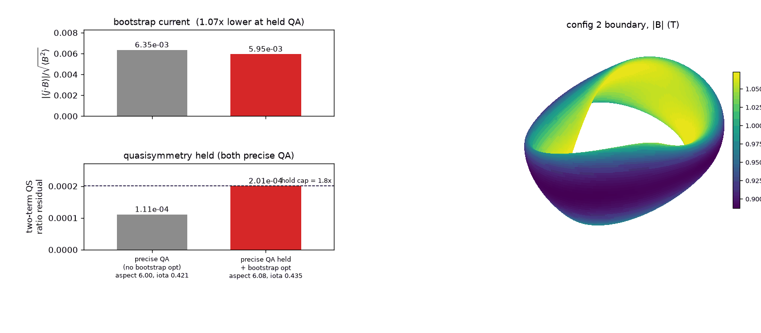

Output figure of examples/optimization/optimize_QA_bootstrap.py.

Example tree

The repository includes a structured examples/ tree:

• examples/tutorials/: notebook-led learning path and a fast output/plot script

• examples/getting_started/: basic API usage (no external reference code required)

• examples/parity/: focused validation scripts against frozen reference fixtures

• examples/transport/: RHSMode=2/3 transport-matrix workflows + upstream scanplot scripts

• examples/autodiff/: autodiff + implicit-diff demonstrations

• examples/optimization/: optimization patterns (may require extras)

• examples/performance/: JIT/performance microbenchmarks

• examples/publication_figures/: publication-style figure generation

• examples/vmex_finite_beta/: finite-beta vmex to dkx radial bootstrap-current and ambipolar-E_r workflow

Run from the repo root:

cd dkx
python examples/tutorials/run_quick_output_and_plot.py
python examples/getting_started/build_grids_and_geometry.py

For a guided classroom-style path, open the notebooks in examples/tutorials in order — a getting-started -> transport -> ambipolar -> optimization arc:

• 00_start_here.ipynb: pick a learning path, verify first-run assets, and map physics goals to example folders.

• 01_cli_outputs_and_plots.ipynb: CLI, output formats, and diagnostics panels.

• 02_transport_and_autodiff.ipynb: RHSMode=2/3 transport matrices and JAX differentiation (deeper: Differentiability).

• 03_bootstrap_redl_and_optimization.ipynb: bootstrap-current/Redl comparisons and optimization objectives (deeper: Optimization Workflows).

• 04_geometry_validation_and_performance.ipynb: analytic/Boozer/VMEC geometry, validation and parity, and CPU/GPU performance pointers (deeper: Performance and differentiability).

For the reduced-model tools that build on these workflows — the monoenergetic-database mode, the variational \(D_{11}\) bounds, and the Shaing-Callen collisionless limit — see Reduced-model capabilities.

The checked catalog examples/workflow_catalog.json mirrors the tables on this page. It records the supported topic folders, first-pass entry points, typical commands, runtime budgets, and whether a workflow requires a local SFINCS Fortran v3 executable.

For a terminal browser over the same catalog:

python examples/list_workflows.py --list-topics
python examples/list_workflows.py --topic bootstrap --long
python examples/list_workflows.py --search "VMEC geometry"

One-command start points

These entries are the shortest useful commands for common workflows. They avoid a local SFINCS Fortran v3 executable unless the command explicitly says it is a frozen-reference or benchmark workflow.

Goal	Entry script	Typical command
Write output files and a diagnostics panel	examples/tutorials/run_quick_output_and_plot.py	python examples/tutorials/run_quick_output_and_plot.py
Inspect HDF5, NetCDF, NPZ, and plotting	examples/getting_started/write_and_plot_multiple_formats.py	python examples/getting_started/write_and_plot_multiple_formats.py
Load VMEC geometry through wout_path	examples/getting_started/write_sfincs_output_vmec.py	python examples/getting_started/write_sfincs_output_vmec.py
Compute a RHSMode=2/3 transport matrix	examples/transport/transport_matrix_rhsmode2_and_rhsmode3.py	python examples/transport/transport_matrix_rhsmode2_and_rhsmode3.py
Differentiate a residual with JAX	examples/autodiff/autodiff_gradient_nu_n_residual.py	python examples/autodiff/autodiff_gradient_nu_n_residual.py
Compare kinetic bootstrap current with Redl	examples/vmex_finite_beta/compare_qs_paper_dkx_redl.py	python examples/vmex_finite_beta/compare_qs_paper_dkx_redl.py --case QA --quick --jax-vs-redl --solve-method auto
Time output formats and memory behavior	examples/performance/benchmark_output_formats.py	python examples/performance/benchmark_output_formats.py --repeats 2
Check a frozen Fortran-v3 output fixture	examples/parity/output_parity_vs_fortran_fixture.py	python examples/parity/output_parity_vs_fortran_fixture.py

Fast tutorial, getting-started, and frozen-fixture parity entries are designed for seconds-scale laptop CPU runs. VMEC, Redl, optimization, and performance entries may take longer; use --quick where available and inspect generated solver metadata before treating a result as quantitative evidence.

Decision map

Use this map when you know the kind of task you need, but not the example folder name.

Starting question	Go here	Why
I want to run one case and plot the output.	examples/tutorials/run_quick_output_and_plot.py	Writes HDF5, NetCDF, NPZ, and a PDF panel in one bounded command.
I want to learn the file formats and CLI/API basics.	examples/getting_started/	Isolates input parsing, output writing, VMEC paths, and plotting.
I need transport coefficients.	examples/transport/	Covers RHSMode=2/3 transport matrices and scan postprocessing.
I need gradients or optimization hooks.	examples/autodiff/ and examples/optimization/	Starts with residual/JVP examples, then moves to QA/QI objectives and promotion gates.
I need bootstrap current or Redl comparisons.	examples/vmex_finite_beta/	Owns the VMEC, Redl, ambipolar-root, and bootstrap-current profile scripts.
I need to validate against SFINCS Fortran v3 behavior.	examples/parity/ and examples/publication_figures/	Provides frozen fixtures and release-facing comparison plot generators.
I need CPU/GPU runtime or memory evidence.	examples/performance/	Benchmarks output formats, JIT, sharding, transport workers, and optional backends.
I recognize an upstream SFINCS input name.	examples/sfincs_examples/	Preserves upstream-style decks for parity and benchmark audits, not first-pass learning.

Application recipe map

Use this table when you know the physics or software task, but not the folder name. The first entry point is the smallest useful run; the research workflow points to the script or notebook that adds production-style validation, convergence, or profiling detail.

Application	Smallest useful entry point	Research workflow
CLI output and diagnostics panel	examples/tutorials/run_quick_output_and_plot.py	examples/getting_started/write_and_plot_multiple_formats.py
Analytic tokamak input	examples/getting_started/write_sfincs_output_tokamak.py	examples/sfincs_examples/tokamak_1species_FPCollisions_noEr/input.namelist
VMEC wout_path input	examples/getting_started/write_sfincs_output_vmec.py	examples/vmex_finite_beta/finite_beta_vmec_to_sfincs.py
RHSMode=2/3 transport matrix	examples/transport/transport_matrix_rhsmode2_and_rhsmode3.py	examples/transport/transport_matrix_rhsmode2_scheme11_and_scheme5.py
Bootstrap current vs Redl	examples/vmex_finite_beta/compare_qs_paper_dkx_redl.py	examples/tutorials/03_bootstrap_redl_and_optimization.ipynb
Ambipolar electric-field scan	examples/vmex_finite_beta/finite_beta_vmec_to_sfincs.py	examples/optimization/evaluate_dkx_promotion_scan.py
Differentiable residual or flux	examples/autodiff/autodiff_gradient_nu_n_residual.py	examples/autodiff/implicit_diff_through_gmres_solve_scheme5.py
VMEC/Boozer/JAX workflow	examples/autodiff/vmex_to_boozer_sfincs_pipeline.py	examples/tutorials/04_geometry_validation_and_performance.ipynb
QA/QI optimization objective	examples/optimization/qa_nfp2_dkx_objectives.py	examples/optimization/QA_optimization_bootstrap_current.py
CPU/GPU timing and output I/O	examples/performance/benchmark_output_formats.py	examples/performance/benchmark_transport_l11_vs_fortran.py
Frozen Fortran-v3 parity check	examples/parity/output_parity_vs_fortran_fixture.py	examples/sfincs_examples/ for retained upstream-style decks

Top-level folder categories

The top-level folders are grouped by user intent. Start with the learning folders when exploring the code, use capability folders for physics or differentiability workflows, and use validation folders when producing parity, performance, or publication evidence. The reference folders are not the recommended first stop for new workflows.

Category	Folders	Use when
learning	examples/tutorials/, examples/getting_started/	You want to learn the CLI, Python API, plots, output formats, and first operator or geometry concepts.
capability	examples/transport/, examples/autodiff/, examples/optimization/, examples/vmex_finite_beta/	You need a specific physics, optimization, VMEC, Redl, bootstrap-current, or differentiability workflow.
validation	examples/parity/, examples/performance/, examples/publication_figures/, examples/paper_benchmarks/	You need parity checks, runtime/memory evidence, CPU/GPU benchmark drivers, regenerated documentation figures, or methods-paper benchmark cases.
reference	examples/data/, examples/sfincs_examples/	You need small shared inputs or recognizable SFINCS Fortran v3 decks for audits and compatibility checks.

Some geometry examples reference public W7-X/HSX/QI equilibrium fixtures by basename. Those multi-megabyte files are fetched from the sfincs-jax-data-v1 release into the local dkx data cache on first use. To prefetch them before running examples, use:

python -m dkx.validation.data_fetch

Writing sfincsOutput.h5 (Python + CLI):

python examples/getting_started/write_sfincs_output_python.py
python examples/getting_started/write_sfincs_output_cli.py

Geometry-specific write-output examples:

python examples/getting_started/write_sfincs_output_tokamak.py
python examples/getting_started/write_sfincs_output_vmec.py

Finite-beta VMEX to kinetic transport

The finite-beta example is a single Python script that reads the bundled input.nfp2_QA_finite_beta VMEC input, runs vmex for a bounded number of fixed-boundary iterations, writes a VMEC-style wout file, and uses that file directly in dkx with geometryScheme=5. It then scans the normalized radial electric field on several flux surfaces, computes ambipolar radial-current roots when each scan brackets them, selects a continuous root branch, and writes a polished PNG/PDF panel with the radial electric-field profile, bootstrap-current radial profile, representative ambipolarity and flux scans in Er, and a VMEC magnetic-field contour plot using a jet colormap. The radial-profile x-axis is normalized toroidal flux, \(\psi_N = r_N^2\), not the square-root radial label used in the input file.

export DKX_VMEX_ROOT=/path/to/vmex  # optional for source checkouts
python examples/vmex_finite_beta/finite_beta_vmec_to_sfincs.py

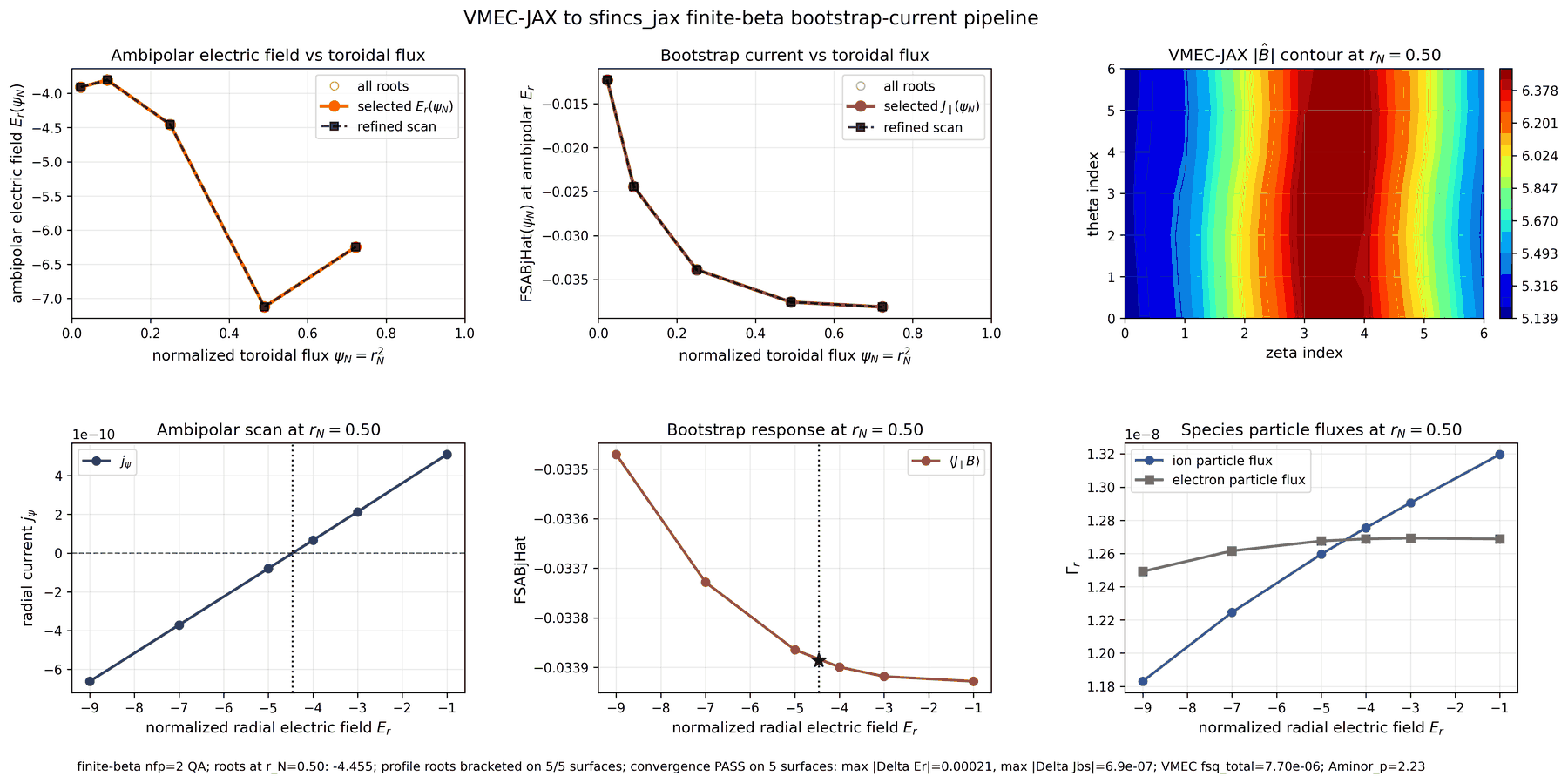
Finite-beta VMEX to dkx example panel. The top row shows the ambipolar radial-electric-field profile versus normalized toroidal flux, the bootstrap-current profile versus normalized toroidal flux, and the sampled VMEC magnetic-field-strength contour. The bottom row shows the representative ambipolarity scan, bootstrap response, and ion/electron particle fluxes versus normalized Er at the selected surface. Open markers show all bracketed roots; filled markers show the selected continuous branch; dashed black markers show the tighter root-bracket convergence scan at the same kinetic grid.

The direct VMEC path does not require a Boozer transform: dkx consumes the generated wout through the same scheme-5 geometry implementation used by file-based VMEC runs. booz_xform_jax remains useful for the separate differentiable Boozer-spectrum workflow described below. This finite-beta script is a primal transport example: it does not differentiate through the VMEX fixed-boundary run, the wout file boundary, scheme-5 geometry evaluation, the SFINCS kinetic solve, or radial postprocessing. Its summary JSON records that boundary in a workflow-contract block, plus radial-profile provenance for the r_N surfaces, plotted \(\psi_N = r_N^2\) values, selected ambipolar branch, all bracketed roots, and convergence-overlay status.

By default the radial profile uses r_N = 0.15, 0.30, 0.50, 0.70, 0.85 and root-neighborhood Er = -9, -7, -5, -3, -1. This spans core-to-edge behavior while avoiding the exact magnetic axis and VMEC boundary, and it spends the expensive solves near the ambipolar branch instead of at far-off electric fields. The checked documentation figure is run at Ntheta=7, Nzeta=7, Nxi=8, NL=6, and Nx=6 with adaptive midpoint refinement of bracketed ambipolar roots until the local Er bracket is no wider than 1.25. The dashed overlay in the top panels uses the same kinetic-space grid on every plotted surface, but refines each bracketed ambipolar root to a local Er bracket width of 0.625. The checked documentation figure passes the default gate, max |Delta Er| <= 0.1 and max |Delta Jbs| <= 5e-4; the measured values are max |Delta Er| = 2.1e-4 and max |Delta Jbs| = 6.9e-7 in the cached documentation run. Use --quick for the smoke-test resolution, and increase --r-n-values, --er-values, and the resolution flags for denser production-quality scans.

The convergence-scan helper reads the cached sfincsOutput.h5 files from the finite-beta example and summarizes which numerical knobs move the ambipolar root and bootstrap current:

python examples/vmex_finite_beta/plot_convergence_scan.py

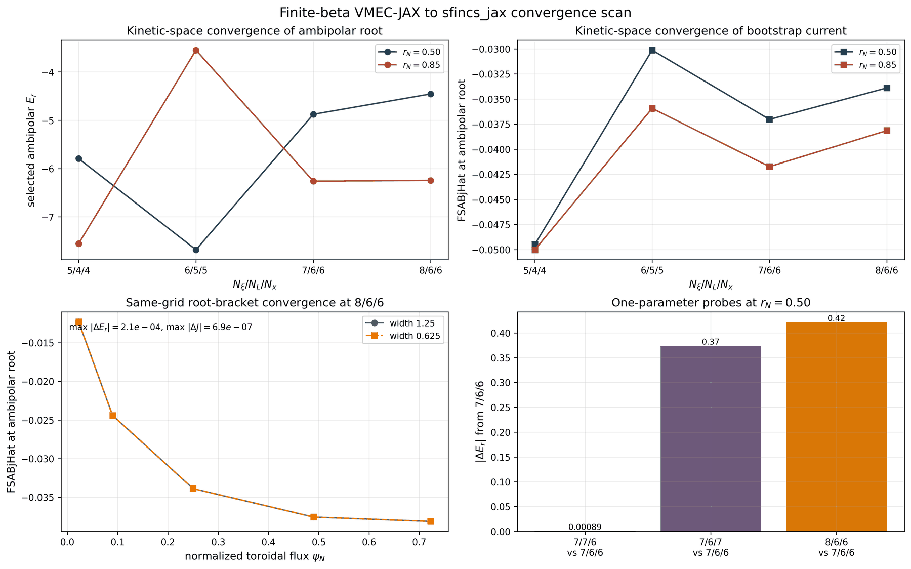
Convergence scan for the finite-beta example. The top panels show that the cached documentation campaign is still sensitive to kinetic-space resolution: moving from 7/6/6 to 8/6/6 changes the selected ambipolar root and bootstrap current, especially at the representative surfaces. The bottom-left panel shows that, once the practical 8/6/6 kinetic grid is fixed, tightening the local ambipolar-root bracket from 1.25 to 0.625 changes the full radial profile by only max |Delta Er| = 2.1e-4 and max |Delta Jbs| = 6.9e-7. The bottom-right panel records one-parameter probes at r_N=0.50: NL=7 is stable, while Nxi=8 and Nx=7 both move the root. Combined Nxi=8,Nx=7 and Nxi=9 probes were too expensive on a single RTX A4000 for this bounded documentation campaign, so this figure is an explicit resolution audit rather than a claim of asymptotic kinetic-space convergence.

DKX / Redl bootstrap-current comparison

The finite-beta directory includes a standalone diagnostic script for the QA and QH SFINCS/Redl benchmarks used in the Zenodo artifact associated with arXiv:2205.02914. The script evaluates the Redl analytic formula on the archived VMEC wout_new_QA_aScaling.nc and wout_new_QH_aScaling.nc files and overlays dkx RHSMode=1 kinetic solves. Use --jax-vs-redl for the first-run path: it plots only dkx and Redl, and does not load or require a SFINCS Fortran v3 executable or archived psiN_*/sfincsOutput.h5 files. If those archived SFINCS Fortran v3 outputs are present in the Zenodo tree, the script can also overlay them as a reference curve without installing or running the Fortran executable. It intentionally makes one plot only: dkx, Redl, and optionally SFINCS Fortran v3, with no NTX or NEOPAX data.

Run a quick QA dkx-versus-Redl diagnostic with no Fortran v3 dependency:

JAX_ENABLE_X64=1 \
python examples/vmex_finite_beta/compare_qs_paper_dkx_redl.py \
  --case QA \
  --quick \
  --jax-vs-redl \
  --solve-method auto \
  --stem qs_paper_qa_jax_redl_quick

For the quasi-helical benchmark, switch the case and stem:

JAX_ENABLE_X64=1 \
python examples/vmex_finite_beta/compare_qs_paper_dkx_redl.py \
  --case QH \
  --quick \
  --jax-vs-redl \
  --solve-method auto \
  --stem qs_paper_qh_jax_redl_quick

This no-Fortran mode still uses the Zenodo input decks and VMEC wout file, and still requires vmex for the Redl algebra; it simply skips every SFINCS Fortran v3 output overlay and metric.

Run the checked 11-surface educational diagnostic used for the same-resolution QA figure:

JAX_ENABLE_X64=1 \
python examples/vmex_finite_beta/compare_qs_paper_dkx_redl.py \
  --case QA \
  --stem qs_paper_qa_same_resolution_11surface \
  --s-values 0.1,0.15,0.25,0.3,0.45,0.5,0.6,0.7,0.75,0.85,0.9 \
  --ntheta 13 --nzeta 13 --nxi 21 --nx 5 \
  --with-errorbars \
  --real-ntheta 15 --real-nzeta 15 \
  --velocity-nxi 25 --velocity-nx 6 \
  --fortran-case-root outputs/qs_paper_fortran_reduced_resolution/QA_Ntheta13_Nzeta13_Nxi21_Nx5 \
  --fortran-errorbar-json docs/_static/figures/vmex_finite_beta/qs_paper_qa_same_resolution_11surface_fortran_errorbars.json \
  --require-same-resolution \
  --solver-tolerance 1e-6 \
  --solve-method auto

Use --case QH --stem qs_paper_qh_same_resolution_11surface, --fortran-case-root outputs/qs_paper_fortran_reduced_resolution/QH_Ntheta13_Nzeta13_Nxi21_Nx5, and the QH Fortran-errorbar JSON sidecar for the quasi-helical configuration. If those local reduced-resolution Fortran sidecars are not present, add --hide-fortran to generate a pure dkx/Redl educational plot. Add --quick for a three-surface smoke plot, or increase the surface list to rerun a denser radial diagnostic.

To re-render a checked figure bundle from its summary JSON without rerunning kinetic solves or requiring local HDF5 sidecars:

python examples/vmex_finite_beta/compare_qs_paper_dkx_redl.py \
  --from-summary-json docs/_static/figures/vmex_finite_beta/qs_paper_qa_same_resolution_11surface.json \
  --stem qs_paper_qa_same_resolution_11surface

Add --jax-vs-redl (alias --hide-fortran) for a pure dkx versus Redl plot. The default --s-values all evaluates all 39 archived surfaces; increase the grid beyond 13 x 13 x 21 x 5 for production accuracy studies.

For an apples-to-apples DKX/SFINCS Fortran v3 figure, use the same-resolution gate:

JAX_ENABLE_X64=1 \
python examples/vmex_finite_beta/compare_qs_paper_dkx_redl.py \
  --case QA --s-values 0.5 \
  --match-fortran-resolution \
  --require-same-resolution \
  --verbose-sfincs \
  --solver-tolerance 1e-6 \
  --solve-method auto

The gate reads the archived Fortran grid and sets the JAX grid to matching Ntheta,Nzeta,Nxi,Nx values before running. If the plotted JAX and Fortran surfaces do not have the same grid, the script fails before writing a public figure. JAX error bars come from --with-errorbars refinement probes. Fortran error bars are plotted only from an explicit --fortran-errorbar-json sidecar; the archived Zenodo outputs contain one Fortran solve per surface, so they do not by themselves define a convergence uncertainty. Use --verbose-sfincs or set DKX_EXAMPLE_VERBOSE=1 for production-grid reruns so the script forwards phase, preconditioner, and Krylov progress messages while setup is running.

The apples-to-apples QA/QH documentation check reruns SFINCS Fortran v3 at the same 13 x 13 x 21 x 5 grid used by the fast JAX documentation solve on 11 surfaces, s = 0.10, 0.15, 0.25, 0.30, 0.45, 0.50, 0.60, 0.70, 0.75, 0.85, 0.90. JAX refinement bars come from independent 15 x 15 x 21 x 5 real-space and 13 x 13 x 25 x 6 velocity-space probes. Fortran bars are one-sided refinement deltas against the archived 25 x 39 x 60 x 7 Fortran v3 outputs. On this same-resolution 11-surface gate, the maximum JAX-vs-Fortran difference is 1.21e-3 for QA and 3.54e-3 for QH. The largest JAX refinement bar is 4.21% for QA and 24.43% for QH, so QH is still a reduced-grid convergence stress test rather than a production-resolution claim.

For this benchmark script, --solve-method auto runs in the runtime/non-autodiff lane (the script sets DKX_IMPLICIT_SOLVE=0). The recorded finite-beta QA/QH figures below remain valid measured evidence, and reruns use the matrix-free auto policy. The script refuses to write nonconverged production-sized diagnostics.

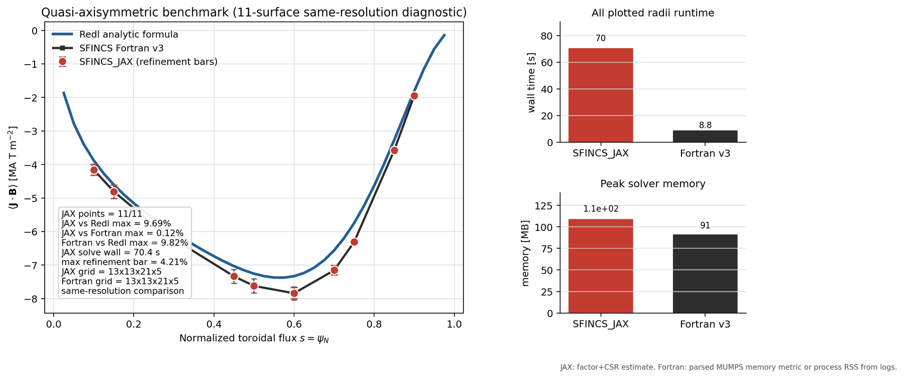
Same-resolution 11-surface QA bootstrap-current gate. The black curve is a local SFINCS Fortran v3 rerun at 13 x 13 x 21 x 5. The red markers are DKX at the same grid, with refinement bars from independent real-space and velocity-space probes. Fortran bars are refinement deltas from the archived 25 x 39 x 60 x 7 Fortran outputs. The maximum JAX-vs-Fortran difference on the 11 surfaces is 1.21e-3.

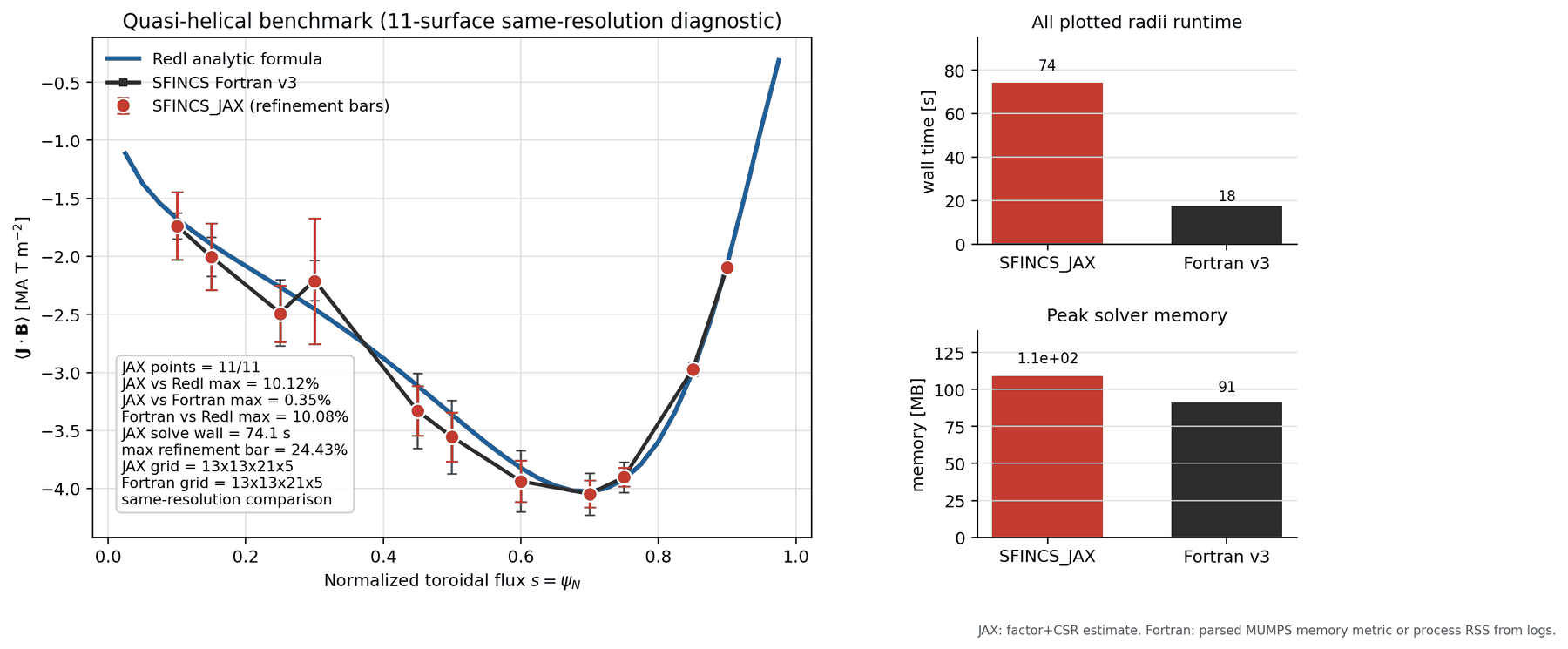
Same-resolution 11-surface QH bootstrap-current gate. The maximum JAX-vs-Fortran difference is 3.54e-3; the larger visible red bars at low radius are JAX velocity-space refinement deltas, not a Fortran/JAX normalization mismatch.

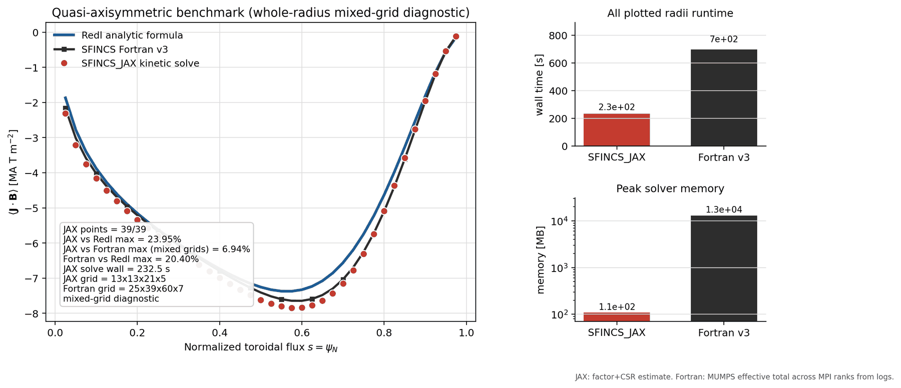
Paper-backed QA bootstrap-current mixed-grid diagnostic. The Redl curve uses the archived VMEC equilibrium and the same polynomial profile contract used in the original SFINCS/Redl comparison. The black curve is the archived SFINCS Fortran v3 output at the paper resolution 25 x 39 x 60 x 7. The red markers are the dkx benchmark auto policy at 13 x 13 x 21 x 5 on the same 39 archived radial surfaces. All solves selected fortran_reduced_pc_gmres and reached the true-residual target. The right panels compare the total solve wall time over all plotted radii and the peak solver-memory metric over those radii. QA completed in 232.5 s with 109 MB JAX solver-memory estimate, versus 696.1 s and 12.96 GB effective total MUMPS factor memory for the archived Fortran v3 run. Max differences are 23.95% versus Redl and 6.94% versus Fortran, so this is a useful reduced-grid diagnostic while the full same-resolution production parity claim remains a separate gate.

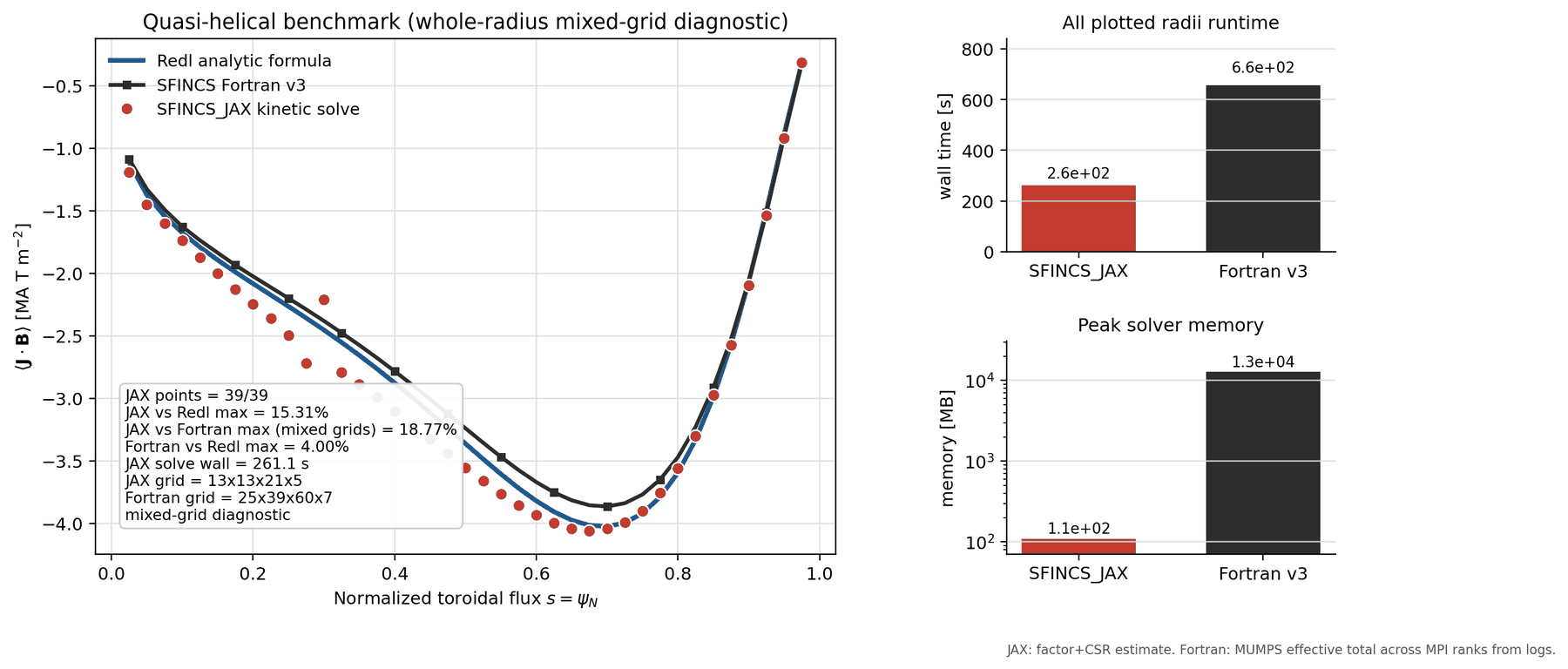
Paper-backed QH bootstrap-current diagnostic with the same whole-radius plotting contract. The QH run is also residual-clean under auto / fortran_reduced_pc_gmres. The JAX scan completed in 261.1 s with 109 MB JAX solver-memory estimate, versus 655.5 s and 12.80 GB effective total MUMPS factor memory for the archived Fortran v3 run. Max differences are 15.31% versus Redl and 18.77% versus Fortran on the reduced JAX grid. This keeps the QH production-resolution convergence lane open; term-level audits point away from a simple stale-radius geometry, radial-gradient conversion, or current-assembly normalization bug, but the production-resolution convergence gate remains the acceptance criterion.

The plotted quantity is the flux-surface-averaged bootstrap current projected along the magnetic field,

\[\langle J\cdot B\rangle .\]

dkx reports the dimensionless diagnostic

\[\widehat{J} = \mathrm{FSABjHat} = \sum_s Z_s\,\mathrm{FSABFlow}_s .\]

For this archived benchmark the SI conversion used by the original SFINCS post-processing script is

\[\langle J\cdot B\rangle_{\rm SFINCS} = \widehat{J}\, \left(437695\right)\left(10^{20}\right)e .\]

The archived SFINCS Fortran v3 and generated dkx outputs both use FSABjHat and the same conversion factor. This makes the plotted Fortran and JAX points a direct output-normalization check, not an extra model fit.

The Redl side follows the Sauter-like analytic bootstrap-current structure of Redl et al. (Phys. Plasmas 28, 022502 (2021), doi:10.1063/5.0012664), using the trapped-particle fraction, local collisionalities, and \(Z_{\rm eff}\) as fit variables. The profile contract is exactly the one in the paper benchmark:

\[n_e(s)=4.13\times 10^{20}(1-s^5)\ {\rm m}^{-3}, \qquad T_e(s)=T_i(s)=12\,{\rm keV}\,(1-s), \qquad Z_{\rm eff}=1 .\]

The effective trapped fraction is

\[f_t = 1-\frac{3}{4}\langle B^2\rangle \int_0^{1/B_{\max}} \frac{\lambda\,d\lambda} {\left\langle \sqrt{1-\lambda B}\right\rangle},\]

and the Redl current is assembled as

\[\langle J\cdot B\rangle_{\rm Redl} = -\frac{G e}{\psi_{\rm edge}(\iota-N)} \left[ (n_eT_e+n_iT_i)L_{31}\frac{d\ln n_e}{ds} +p_e(L_{31}+L_{32})\frac{d\ln T_e}{ds} +p_i(L_{31}+\alpha L_{34})\frac{d\ln T_i}{ds} \right],\]

where \(s=\psi_N\) and \(N=N_{\rm fp}\,\mathrm{helicity\_n}\). The QA benchmark uses helicity_n = 0 with wout_new_QA_aScaling.nc; the QH benchmark uses helicity_n = -1 with wout_new_QH_aScaling.nc. The fitted functions \(L_{31}\), \(L_{32}\), \(L_{34}\), and \(\alpha\) are the Redl/Sauter bootstrap coefficients implemented in vmex.redl_bootstrap.redl_bootstrap_jdotb and used here only for the analytic Redl curve.

This check also exercises SFINCS v3 radial-coordinate compatibility: the archived inputs specify inputRadialCoordinate = 1 and psiN_wish, so dkx must select the VMEC surface from \(s=\psi_N\) rather than assuming an rN_wish input. The associated unit tests cover this psiN_wish path and the Er to dPhiHat/dpsiHat conversion.

Main references for this diagnostic are Redl et al. 2021 for the analytic bootstrap fit, Sauter et al. 1999/2002 for the original tokamak fit structure, Landreman et al. 2014 for the SFINCS kinetic model, and the arXiv:2205.02914 Zenodo benchmark artifact for the QA/QH comparison data. See References and related work for the full citation list and links.

Plotting a generated or frozen output file:

dkx --plot sfincsOutput.h5
python examples/getting_started/plot_sfincs_output.py

Matrix-free linear solve demo (using frozen PETSc binaries):

python examples/parity/solve_fortran_matrix_with_gmres.py
python examples/autodiff/autodiff_gradient_nu_n_residual.py

Transport matrices (RHSMode=2/3)

Upstream v3 uses RHSMode=2 and RHSMode=3 to compute transport matrices by looping over multiple right-hand sides (whichRHS) and assembling a matrix from diagnostic moments of the solved distribution.

dkx provides both a Python driver and a CLI:

python examples/transport/transport_matrix_rhsmode2_and_rhsmode3.py
dkx transport-matrix-v3 --input input.namelist --out-matrix transportMatrix.npy

Upstream postprocessing (utils/)

The mature SFINCS ecosystem includes a set of plotting scripts under utils/. dkx vendors these scripts in examples/sfincs_examples/utils/ and can run them non-interactively:

dkx postprocess-upstream --case-dir /path/to/case --util sfincsScanPlot_1 -- pdf

For a small end-to-end transport-matrix postprocessing workflow, generate a matrix and then call the supported upstream utility wrapper:

dkx transport-matrix-v3 --input input.namelist --out-matrix transportMatrix.npy
dkx postprocess-upstream --case-dir . --util sfincsScanPlot_1 -- --pdf

Some advanced examples require optional dependencies:

pip install optax

Optimization + figures

The retained optimization examples focus on a QA nfp=2 workflow: a fast differentiable proxy objective, an editable VMEX-style QA script with an optional bootstrap-current term, and promotion audits from completed dkx scan-er outputs.

python examples/optimization/qa_nfp2_dkx_objectives.py --objective balanced --steps 20
python examples/optimization/QA_optimization_bootstrap_current.py

Optional ecosystem solver-library comparisons are research-lane material rather than stable user examples. The retained examples use the in-tree JAX differentiable geometry and optimization helpers.

Implicit differentiation through solves

An important differentiability capability is implicit differentiation through a linear solve (A x = b) without backpropagating through Krylov iterations. dkx provides a small helper based on jax.lax.custom_linear_solve and demonstrates it here:

python examples/autodiff/implicit_diff_through_gmres_solve_scheme5.py

Edit the SOLVE_METHOD parameter at the top of the script to route the solve through the auto, block_tridiagonal, or gmres tier.

VMEC-to-Boozer Differentiable Geometry Workflow

For optional vmex and booz_xform_jax installations, this example checks a public differentiable geometry workflow into dkx:

python examples/autodiff/vmex_to_boozer_sfincs_pipeline.py

The script first prints the optional-backend status and runs a dependency-free Boozer-proxy gradient gate. When vmex and booz_xform_jax are installed and a VMEC wout resolves, it then reports a Boozer-spectrum geometry proxy, its JAX gradient, a centered finite-difference gradient, and a few scalar optimization steps. Edit the WOUT_PATH, SURFACE, MBOZ, and NBOZ parameters at the top (or set DKX_VMEX_WOUT) to change the input. It is a fast research workflow gate for JAX-native geometry coupling; it is not a full kinetic transport optimization solve.

The dependency-free backend status and gradient gate always run first, and the workflow summary JSON records shallow backend availability, differentiability labels, the exact geometry-proxy gradient claim, deferred kinetic-gradient work, and a no-overclaim gate that forbids presenting this lane as full VMEC-boundary-to-SFINCS transport differentiation.

Parallel and scaling examples

The legacy transport-worker scaling benchmark was deleted with the legacy pipeline. Host-device parallelism for canonical runs is configured through the DKX_CORES/DKX_CPU_DEVICES environment knobs (Parallelism); single-case sharded RHSMode=1 scaling remains a research lane rather than a stable example.

Note

geometryScheme=5 (VMEC) and analytic tokamak geometryScheme=1 are supported public examples. dkx does not expose a separate Miller-parameter geometry mode in the public CLI/API, so tokamak examples use the supported analytic Boozer tokamak path instead.

The autodiff examples build cached operators, treat scalar inputs such as \(\\nu_n\) as differentiable parameters, and use custom_linear_solve where implicit gradients are the memory-efficient path. This is the recommended pattern for gradients without backpropagating through every Krylov iteration.

Upstream SFINCS example inputs

For convenience, dkx vendors the upstream-style SFINCS-v3 example suite in examples/sfincs_examples/. These files are recognizable reference points for SFINCS users and support compatibility audits. A best-effort runner is provided:

python examples/sfincs_examples/run_dkx.py --write-output