Physics reference: the radially local drift-kinetic model
This page is the physics reference for the canonical dkx stack. It derives the radially local, linearized drift-kinetic equation (DKE) that the code solves, states the SFINCS normalization conventions, and maps every term onto the module that implements it. The equations quoted here are the forms the code assembles (the implementing module and operator are named in the Where in the code boxes), not a paraphrase of an external note.
For textbook background see Helander & Sigmar, Collisional Transport in Magnetized Plasmas (2002); for the SFINCS model specifically see Landreman, Smith, Mollén & Helander, Phys. Plasmas 21, 042503 (2014). Full citations are collected in References and related work; the block linear-algebra view is in Drift-kinetic equation and system of equations and Numerics and algorithms; the geometry inputs are in Geometry models and loading.
Governing equation and the \(f_0+f_1\) split
dkx solves for the non-adiabatic first-order distribution \(f_{s1}\) of each kinetic species \(s\) on a single flux surface, holding the radial profiles and their gradients fixed (the radially local approximation). The full distribution is split
where the second exponential is present only when the flux-surface potential variation \(\Phi_1(\theta,\zeta)\) is enabled (otherwise \(f_{s0}\) is a pure Maxwellian). The velocity coordinates are the normalized speed and the pitch-angle cosine
The steady linearized DKE is written schematically as
with a source \(S_s\) built from the radial thermodynamic drives and the inductive field. Each term is derived and mapped to code below.
Where in the code
The whole operator is the single consolidated
dkx.drift_kinetic.KineticOperator. Its matrix-free action on
the distribution block is KineticOperator.apply_f;
the term-by-term pieces are the _streaming_mirror, _exb,
_er_xidot, and _er_xdot methods; the drive \(S_s\) is
KineticOperator.rhs. Build one from a namelist
with dkx.drift_kinetic.kinetic_operator_from_namelist().
Normalization: \(\Delta\), \(\alpha\), \(\nu_n\)
SFINCS works with hatted (dimensionless) fields. Lengths are in a reference \(\bar R\), magnetic fields in \(\bar B\), so that \(\hat B = B/\bar B\) and \(\hat\psi = \psi/(\bar B\bar R^2)\). Three scalar parameters set the physical scale of the drift-kinetic ordering:
\(\Delta\) (
Delta) is the drift ordering parameter — the ratio of a thermal gyroradius to \(\bar R\). It multiplies every drift term (\(\mathbf{v}_E\), \(\mathbf{v}_m\), and the radial fluxes).\(\alpha\) (
alpha) converts the normalized potential to a normalized energy; it appears wherever the electrostatic potential enters (\(E\times B\) drive, \(\Phi_1\) Boltzmann factor, quasineutrality).\(\nu_n\) (
nu_n) is the overall collision-frequency normalization multiplying the collision operator.
These are the Delta, alpha, nu_n namelist inputs; they are written
verbatim into sfincsOutput.h5 (see Outputs (HDF5, NetCDF4, and NPZ)). For monoenergetic
(RHSMode=3) runs the physical collisionality and electric field are supplied
instead as nuPrime and EStar:
with \(\hat G\), \(\hat I\) the covariant Boozer flux functions, \(\iota\) the rotational transform, and \(\hat B_0\) the \((0,0)\) Fourier mode of \(\hat B\). See Normalizations and units for the radial- coordinate conventions and the full unit table.
Streaming and mirror terms
Parallel streaming and the mirror force are the collisionless backbone of the DKE. In the Legendre representation \(f_{s1}=\sum_L f_{sL}(x,\theta,\zeta)P_L(\xi)\), the parallel-gradient operator is
and streaming couples each Legendre mode \(L\) to its neighbours \(L\pm 1\) through the recursion \(\xi P_L = \frac{L+1}{2L+3}P_{L+1} + \frac{L}{2L-1}P_{L-1}\):
The mirror force \(\mathcal{M}\) carries the same \(L\pm1\) structure with the geometric prefactor
the upper/lower couplings scaled by \((L+2)\) and \(-(L-1)\) respectively. These two terms are always present.
Where in the code
KineticOperator._streaming_mirror. The Legendre
coupling coefficients \(\frac{L+1}{2L+3}\) and \(\frac{L}{2L-1}\)
are dkx.phase_space.legendre_coupling_upper() /
legendre_coupling_lower. The same coefficients build the analytic
block-tridiagonal factorization in KineticOperator.legendre_blocks.
\(E\times B\) drift
The equilibrium radial electric field \(E_r=-d\Phi_0/dr\) produces an \(E\times B\) advection in the angular directions. Its diagonal-in-\(L\) prefactors are
where \(\hat D\) is the Jacobian factor and \(\hat B_\theta\), \(\hat B_\zeta\) are covariant components. The denominator \(\mathcal{B}\) encodes the trajectory model:
default (full) trajectories: \(\mathcal{B} = \hat B^2\);
DKES trajectories (
useDKESExBDrift = .true.): \(\mathcal{B} = \langle \hat B^2\rangle\), the flux-surface average. This is the monoenergeticincompressible\(E\times B\) used for DKES-style benchmarks.
Where in the code
KineticOperator._exb and _exb_coefficients.
The useDKESExBDrift switch selects
\(\hat B^2\) vs \(\langle \hat B^2\rangle\) (fsab_hat2).
Radial-electric-field energy and pitch-angle drifts
The full trajectory model adds two more \(E_r\)-driven terms that couple
\(L\leftrightarrow L, L\pm 2\). The \(\dot\xi\,\partial_\xi\) term
(enabled by includeElectricFieldTermInXiDot) has coefficient
with the diagonal Legendre weight \(\frac{L(L+1)}{(2L-1)(2L+3)}\) and
\(L\pm2\) couplings. The \(\dot x\,\partial_x\) term (enabled by
includeXDotTerm) acts through the dense speed operator \(x\,\partial_x\)
with prefactor
Both terms vanish when \(d\hat\Phi/d\hat\psi=0\), so an \(E_r=0\) run reduces to the collisionless streaming/mirror plus collisions.
Where in the code
KineticOperator._er_xidot and _er_xdot. The trajectory model is therefore encoded entirely by
three flags: useDKESExBDrift (DKES \(E\times B\)),
includeElectricFieldTermInXiDot, and includeXDotTerm. The tangential
magnetic drift terms (magneticDriftScheme 1–9, matching the Fortran
select case blocks) are assembled in drift_kinetic.py; the full
trajectory here means the full \(E_r\) terms.
Thermodynamic and inductive drives
The source \(S_s\) collects the free-energy drives. The radial-gradient drive, projected onto Legendre modes \(L=0\) (weight \(4/3\)) and \(L=2\) (weight \(2/3\)), is
with the geometric factor
\(\hat g_2 = \hat D\,(\hat B_\zeta\,\partial_\theta\hat B -
\hat B_\theta\,\partial_\zeta\hat B)/\hat B^3\). The inductive drive
(\(L=1\)) is proportional to the parallel electric field
\(\hat E_\parallel\) (EParallelHat) times \(\hat B\):
For the electrostatic (radial-gradient) part, the \(d\hat\Phi/d\hat\psi\) piece is dropped in transport-matrix modes so each drive can be isolated (see below).
Where in the code
KineticOperator.rhs. Transport-matrix RHS column
overwrites (whichRHS) are handled by _with_rhs_settings.
Collision operators
dkx implements three collision models, selected by
collisionOperator: the two SFINCS v3 operators (full Fokker–Planck and
pitch-angle scattering) plus the momentum- and energy-conserving improved
Sugama model operator (collisionOperator = 3), a research extension beyond
Fortran v3.
Pitch-angle scattering (collisionOperator = 1)
The Lorentz (pitch-angle-scattering, PAS) operator is diagonal in \((\theta,\zeta,x)\) and in the Legendre index, with the classic \(L(L+1)\) eigenstructure:
where the deflection frequency \(\hat\nu_D^s(x)\) is built from the error function and the Chandrasekhar function
PAS is block-diagonal in \(L\), which is what makes the tier-1 structured solve applicable (Numerics and algorithms).
Where in the code
The pitch-angle-scattering operator lives in dkx.collisions and
is applied inside KineticOperator.apply_f; the \(L(L+1)\) factor is
dkx.phase_space.lorentz_eigenvalues(), and the deflection
frequency and Chandrasekhar function are helpers in the same module.
Full linearized Fokker–Planck (collisionOperator = 0)
The full linearized Landau operator adds, on top of the pitch-angle deflection, the energy-scattering (test-particle) piece and the field-particle back-reaction that restores momentum and energy conservation. For each species pair and Legendre mode it is a dense matrix in the speed grid:
The field-particle term \(R_L\) is expressed through the Rosenbluth potentials \(H\), \(G\) of a Maxwellian target. The code builds, for each \(L\), the speed integrals that give \(H\), \(dH/dx\), and \(d^2G/dx^2\), then maps them back to the collocation grid:
and analogously for the derivative and second-derivative potentials. Momentum
and energy conservation are structural — they follow from using the exact
linearized field term (there is no ad-hoc moment-restoring projection unless the
optional Krook drag is requested). The dense speed coupling of \(C^{FP}\)
is the dominant cost of a multi-species Fokker–Planck run.
Where in the code
The full Fokker–Planck operator and its Rosenbluth-potential speed integrals
live in dkx.collisions, ported from the Landreman–Ernst
speed-grid treatment
(arXiv:1210.5289). Both the
pitch-angle-scattering and Fokker–Planck blocks are applied through
KineticOperator.apply_f.
Improved Sugama model operator (collisionOperator = 3)
A research extension beyond Fortran v3: the momentum- and energy-conserving
improved linearized model collision operator of Sugama et al.
(Phys. Plasmas 26, 102108, 2019), built with the moment-based field-particle
construction of Frei, Ernst & Ricci (Phys. Plasmas 29, 093902, 2022). The
test-particle part reuses the Fokker–Planck deflection and energy-diffusion
kernels; the field-particle back-reaction is a low-rank moment term (L=0
particle/energy, L=1 parallel momentum) whose coefficients cancel the
test-particle moment functionals algebraically, so conservation is exact at
the collocation level. It assembles into the same per-L dense speed blocks
as the Fokker–Planck operator.
Where in the code
The improved Sugama construction lives in dkx.collisions
next to the Fokker–Planck blocks and shares the same matvec
(apply_fokker_planck_v3), applied through KineticOperator.apply_f.
Flux-surface potential variation \(\Phi_1\) and quasineutrality
When includePhi1 = .true. the electrostatic potential carries a
flux-surface variation,
which enters the leading-order distribution as the Boltzmann factor \(f_{s0}=f_{sM}\exp(-Z_s\alpha\Phi_1/\hat T_s)\). The additional unknown \(\Phi_1(\theta,\zeta)\) is closed by quasineutrality, and the gauge freedom is fixed by \(\langle\Phi_1\rangle=0\):
Two closures are supported: quasineutralityOption = 1 (full Boltzmann
response, summing all kinetic species) and quasineutralityOption = 2 (the
EUTERPE-style single-species adiabatic form). Because \(f_{s0}\) depends
nonlinearly (exponentially) on \(\Phi_1\), the coupled kinetic +
quasineutrality system is solved by a warm-started Newton iteration; the whole
map is differentiable through the implicit-function theorem.
Where in the code
The quasineutrality rows and the \(\langle\Phi_1\rangle=0\) Lagrange row
are KineticOperator._quasineutrality_rows; the
\(\Phi_1\)-in-kinetic coupling is _add_phi1_in_kinetic; the \(\Phi_1\)-in-collision poloidal density
factor \(n_s e^{-Z_s\alpha\Phi_1/\hat T_s}\) is applied in apply_f.
The nonlinear Newton driver is dkx.phi1.solve_phi1(), with the
differentiable variant
dkx.phi1.phi1_state(). readExternalPhi1 treats
\(\Phi_1\) as a fixed external field: a linear solve (no Newton
iteration) routed through dkx.run.run_profile().
Moments, fluxes, and transport coefficients
The physical outputs are velocity-space and flux-surface-average moments of the solved \(f_{s1}\). All radial fluxes are computed natively on \(\nabla\hat\psi\) and then converted to the \(\psi_N\), \(\hat r\), \(r_N\) variants (Outputs (HDF5, NetCDF4, and NPZ)).
Particle and heat flux (magnetic drift). The radial flux carried by the magnetic drift uses the geometric factor \(\hat g_{vm} = (\hat B_\theta\,\partial_\zeta\hat B - \hat B_\zeta\,\partial_\theta\hat B)/\hat B^3\) and Legendre weights \(8/3\) (\(L=0\)) and \(4/15\) (\(L=2\)):
These are the particleFlux_vm_psiHat / heatFlux_vm_psiHat outputs. The
_vm0 variants use only \(f_{s0}\); the \(E\times B\) flux family
(_vE) uses the analogous factor
\((\hat B_\theta\,\partial_\zeta\Phi_1 - \hat B_\zeta\,\partial_\theta\Phi_1)/\hat B^2\)
(note the \(\hat B^2\) denominator, a genuine physical difference from the
magnetic-drift \(\hat B^3\)).
Parallel flow and bootstrap current. The \(L=1\) moment gives the parallel flow and, summed over species with the charge weight, the bootstrap current \(\langle\mathbf{j}\cdot\mathbf{B}\rangle\):
FSABjHat is the neoclassical bootstrap current; jHat is the parallel
current density on the \((\theta,\zeta)\) grid.
Monoenergetic transport matrix and Onsager symmetry. For RHSMode=2 (a
\(3\times3\) thermal transport matrix) and RHSMode=3 (a
\(2\times2\) monoenergetic/DKES matrix), the code loops over the drive
columns and assembles \(L_{ij}\) mapping the thermodynamic forces (radial
gradient drive, parallel electric field) to the responses (radial flux, parallel
flow). The shared \(\hat g_+ = \hat G + \iota\hat I\) and
\(b_0/\hat G^2\) normalization structure is what enforces the Onsager
symmetry \(L_{12}=L_{21}\); the examples/transport/transport_coefficients.py script
prints the measured Onsager asymmetry as a check. The classic result is that in
a non-axisymmetric field the radial coefficient \(L_{11}\) (\(D_{11}\)-
like) grows like \(1/\nu\) at low collisionality:
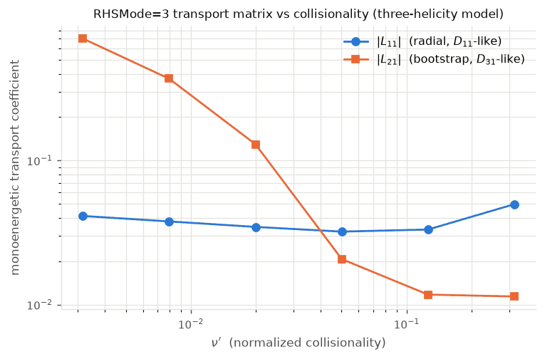
Monoenergetic (RHSMode=3) transport-matrix entries versus normalized
collisionality \(\nu'\) for a three-helicity model field. \(|L_{11}|\)
(radial, \(D_{11}\)-like) rises at low \(\nu'\) — the characteristic
\(1/\nu\) neoclassical regime of a non-axisymmetric configuration —
while \(|L_{21}|\) (bootstrap, \(D_{31}\)-like) tracks the parallel
response. Reproduce with python docs/figures/generate_docs_figures.py.
Where in the code
Magnetic-drift fluxes: dkx.moments.vm_flux_moments(); RHSMode-1 per-species table including FSABjHat and
FSABFlow: dkx.moments.rhsmode1_moments();
\(E\times B\) flux: electric_drift_flux_moments;
transport matrix: dkx.moments.transport_matrix_from_flux_arrays().
Ambipolarity and the radial electric field
Unlike a tokamak, a stellarator field is not intrinsically ambipolar: the ion and electron radial fluxes depend independently on \(E_r\), so a net radial current would flow unless \(E_r\) self-adjusts to the ambipolar root
dkx evaluates \(J_r\) at a given \(E_r\) with one drift-kinetic
solve and finds the root with a bracket-expanding Brent solver that mirrors
SFINCS Fortran v3 ambipolarSolver.F90 (option 2), classifying each root as
ion, electron, or unstable. The root is also exposed as a differentiable
quantity: \(dE_r/dp\) for any profile parameter \(p\) follows from the
implicit-function theorem applied to \(J_r(E_r,p)=0\), so jax.grad flows
through the ambipolar \(E_r\).
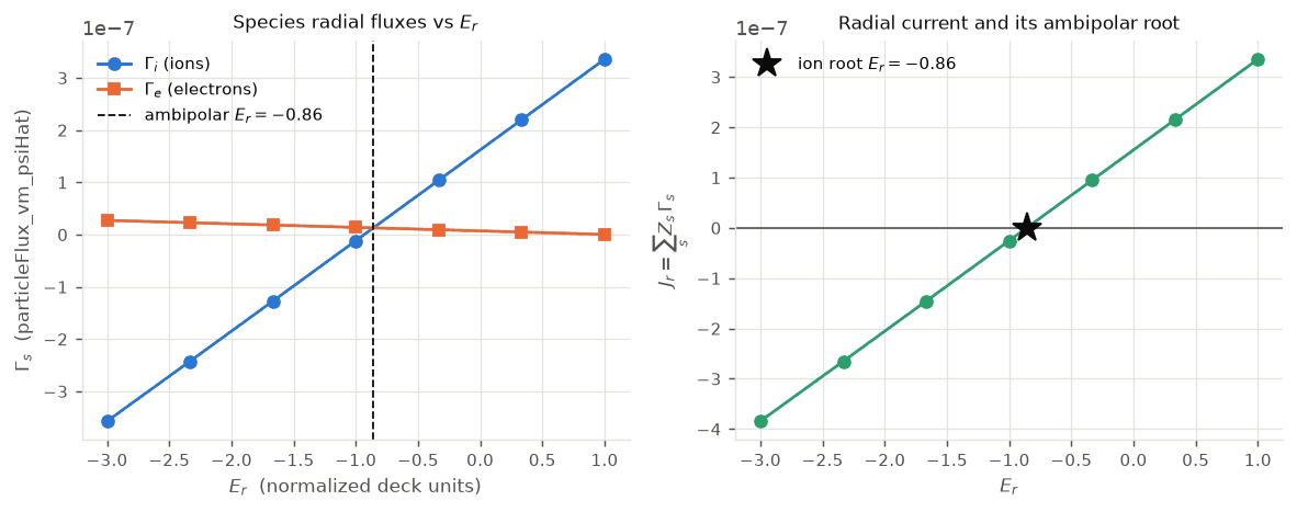
Left: ion and electron radial fluxes \(\Gamma_s(E_r)\) for a model
stellarator with an ion+electron pair. Right: the radial current
\(J_r=\sum_s Z_s\Gamma_s\) and its ambipolar (ion) root. Reproduce with
python docs/figures/generate_docs_figures.py.
Where in the code
Radial current \(J_r=\sum_a Z_a\Gamma_a\):
dkx.er.radial_current(); Brent root find and
classification: dkx.er.find_ambipolar_er() with the
_brent kernel; differentiable root:
dkx.er.ambipolar_er() (implicit-function theorem through
solvax.implicit.root_solve). See examples/vmex_finite_beta/ambipolar_er_scan.py.
Classical (collisional) transport
In addition to the neoclassical fluxes above, the code evaluates the classical
(finite-gyroradius, collisional) particle and heat fluxes from the friction
forces of the linearized collision operator, following the upstream SFINCS
classical-radial-fluxes note (see Upstream SFINCS sources and primary literature). These are written as
classicalParticleFlux* / classicalHeatFlux* for geometries that provide
the \(|\nabla\hat\psi|^2\) metric (VMEC scheme 5 and Boozer .bc schemes
11/12).
Equation-to-code map
Physics term |
Canonical implementation |
Enabling input |
|---|---|---|
Streaming \(v_\parallel\mathbf{b}\cdot\nabla f\) + mirror |
|
always on |
\(E\times B\) drift |
|
|
\(E_r\) pitch-angle drift (\(\dot\xi\partial_\xi\)) |
|
|
\(E_r\) energy drift (\(\dot x\partial_x\)) |
|
|
Thermodynamic + inductive drives \(S_s\) |
|
profile gradients, |
Pitch-angle scattering |
Pitch-angle scattering in |
|
Full Fokker–Planck (Rosenbluth) |
Full Fokker–Planck in |
|
\(\Phi_1\) / quasineutrality |
|
|
Fluxes, |
|
|
Ambipolar \(E_r\) |
|
|
Flux-surface geometry |
|
|
Upstream derivations
The long-form derivations are documented in the peer-reviewed SFINCS paper (Landreman, Smith, Mollén, and Helander, Phys. Plasmas 21, 042503 (2014), doi:10.1063/1.4870077) and in the unpublished upstream SFINCS project documents archived at github.com/landreman/sfincs (cited from Upstream SFINCS sources and primary literature). The pieces most relevant to this reference are:
the version-3 technical documentation — the master reference for the operator and normalization;
the single-species and multi-species technical documentation — the drive and collision derivations;
the Fokker–Planck operator implementation note — the Rosenbluth-potential field term;
the \(\Phi_1\) implementation and “effects on fluxes” notes — the \(\Phi_1\)/quasineutrality closure and its effect on the flux definitions;
the transport-matrix / Beidler-matrix note — the transport-coefficient correspondence;
the classical-radial-fluxes and DKES notes — classical fluxes and DKES-limit compatibility.