Geometry models and loading

dkx solves a radially local neoclassical kinetic problem on a single flux surface, so geometry is not an incidental input: the magnetic field strength \(\hat B(\theta,\zeta)\), its derivatives, the Jacobian factor \(\hat D\), and the covariant/contravariant field components set the coefficients of the streaming, mirror, \(E\times B\), and magnetic-drift terms (Physics reference: the radially local drift-kinetic model), as well as the flux-surface averages used in every diagnostic.

All geometry is consolidated in the single canonical module dkx.magnetic_geometry, which mirrors the Fortran v3 geometry.F90 (initializeGeometry / computeBHat_* / setBoozerCoordinates / computeBIntegrals). Every geometry source produces the same normalized container, dkx.magnetic_geometry.FluxSurfaceGeometry, on a (Ntheta, Nzeta) grid.

Supported geometry schemes

geometryScheme	Model	Coordinates	Constructor
1	Analytic three-helicity straight-field-line model	Boozer	FluxSurfaceGeometry.from_scheme(1, ...)
2	LHD standard reduced model (Beidler 2011 table)	Boozer	from_scheme(2, ...)
3	LHD inward-shifted reduced model	Boozer	from_scheme(3, ...)
4	W7-X standard reduced model	Boozer	from_scheme(4, ...)
5	VMEC wout equilibrium (ASCII or netCDF)	VMEC	from_vmec(...) via read_vmec_wout
11	Boozer .bc file, stellarator-symmetric	Boozer	from_boozer(...) via read_boozer_bc
12	Boozer .bc file, non-stellarator-symmetric	Boozer	from_boozer(...) via read_boozer_bc
13	Namelist-supplied Boozer \(|B|\) spectrum (optimization path)	Boozer	from_fourier(...) (differentiable)

The namelist entry point dkx.drift_kinetic.KineticOperator.from_namelist() builds geometry schemes {1, 2, 3, 4, 5, 11, 12} directly from an input.namelist. Scheme 13 is reachable through the differentiable from_fourier constructor in Python; parsing bmnc/bmns amplitudes from a namelist is deferred (see Deferrals below).

The analytic reduced models (schemes 2/3/4) use the harmonic tables from Beidler et al., Nucl. Fusion 51, 076001 (2011). For example, the W7-X standard model (scheme 4) has five field periods and the field strength shown below.

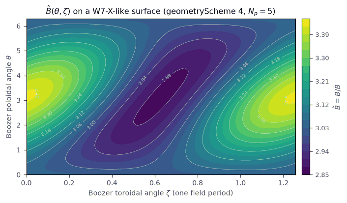
\(\hat B(\theta,\zeta) = B/\bar B\) on one field period of a W7-X-like flux surface, evaluated analytically from FluxSurfaceGeometry.from_scheme(4, ...) (geometryScheme = 4). The low-field “bean” region and the high-field lobes set the trapped-passing boundary that dominates low-collisionality transport. Reproduce with python docs/figures/generate_docs_figures.py.

Boozer vs VMEC coordinates and the \(|B|\) Fourier representation

The analytic and .bc schemes work in Boozer coordinates, where the field strength is a Fourier series in the Boozer angles

\[\hat B(\theta,\zeta) = \sum_{m,n} \hat B_{mn}\,\cos\!\bigl(m\theta - N_p\,n\,\zeta\bigr) \;\;[+\ \text{sine terms for non-symmetric fields}],\]

with \(N_p\) the number of field periods (the n index does not carry the period factor, matching the Fortran boozer_bmnc(m,n) convention). The covariant components reduce to the flux functions \(\hat B_\theta = \hat I\), \(\hat B_\zeta = \hat G\) plus the field- period structure, which is why Boozer geometry is the natural setting for the drift coefficients and for monoenergetic (RHSMode>3) runs.

The retained harmonics follow the representable-mode policy imposed by the discrete \((\theta,\zeta)\) grid, matching the v3 Jacobian assembly at a given resolution:

\[0 \le m \le \left\lfloor \frac{N_\theta}{2}\right\rfloor, \qquad |n| \le \left\lfloor \frac{N_\zeta}{2}\right\rfloor,\]

with the expected Nyquist exclusions for sine/cosine pairs. This truncation matters numerically: the resolved harmonic content changes both the geometric coefficients and the trapped-passing boundary structure.

For geometryScheme = 5 the equilibrium is a VMEC wout file. VMEC stores the field in its own flux coordinates and on a radial mesh, so the loader interpolates the requested surface (half/full-mesh with the v3 finite-difference conventions) and reconstructs \(\hat B\), its derivatives, and the \(|\nabla\hat\psi|^2\) metric used by the classical fluxes and the Sugama-form magnetic drifts.

The differentiable geometry path

Two constructors are pure JAX and safe to jit / grad: FluxSurfaceGeometry.from_scheme (analytic schemes 1–4) and FluxSurfaceGeometry.from_fourier (a Boozer \(|B|\) spectrum). The latter is the geometry entry point for optimization loops: gradients with respect to the spectral amplitudes bmnc/bmns flow through \(\hat B\), \(\hat D\), and the flux-surface averages.

import jax
import jax.numpy as jnp
from dkx.magnetic_geometry import FluxSurfaceGeometry

theta = jnp.linspace(0.0, 2.0 * jnp.pi, 24, endpoint=False)
zeta = jnp.linspace(0.0, 2.0 * jnp.pi / 5.0, 20, endpoint=False)

# A tiny W7-X-like |B| spectrum: (m, n) modes and cosine amplitudes in Bbar units.
m = jnp.asarray([0, 0, 1, 1])
n = jnp.asarray([0, 1, 0, 1])
bmnc = jnp.asarray([3.0, 0.05, -0.02, -0.04])

def objective(amps):
    geom = FluxSurfaceGeometry.from_fourier(
        theta=theta, zeta=zeta, bmnc=amps, m=m, n=n,
        n_periods=5, iota=0.87, g_hat=-17.885, i_hat=0.0,
    )
    # e.g. minimize mirror-ripple-like content in |B|
    return jnp.mean((geom.b_hat - jnp.mean(geom.b_hat)) ** 2)

value, grad = jax.value_and_grad(objective)(bmnc)

Grid truncation of unrepresentable modes is applied by zeroing amplitudes, which keeps array shapes static under jit. A worked differentiable-geometry gradient check is in examples/autodiff/differentiable_geometry_gradients.py.

The FluxSurfaceGeometry container

The operator does not carry an opaque geometry object; the solve path works with explicitly normalized arrays collected in the frozen dataclass dkx.magnetic_geometry.FluxSurfaceGeometry. Its fields follow the SFINCS v3 sfincsOutput.h5 names (BHat \(\to\) b_hat, DHat \(\to\) d_hat, …):

• scalars: n_periods, b0_over_bbar, iota, g_hat (GHat), i_hat (IHat);

• (Ntheta, Nzeta) arrays: b_hat and its \(\theta\)/\(\zeta\) derivatives, d_hat, and the co/contravariant components b_hat_sub_theta/zeta, b_hat_sup_theta/zeta with their derivatives;

• radial/drift arrays (populated from neighbouring surfaces for .bc/VMEC input) and the optional gpsipsi \(=|\nabla\hat\psi|^2\) metric.

Two flux-surface averages are methods on the container: vprime_hat (\(\hat V' = \sum_{ij} w^\theta_i w^\zeta_j/\hat D_{ij}\)) and fsab_hat2 (\(\langle\hat B^2\rangle\)).

Where in the code

dkx.magnetic_geometry. Constructors: FluxSurfaceGeometry.from_scheme (analytic 1–4, magnetic_geometry.py), from_fourier (differentiable Boozer spectrum, magnetic_geometry.py), from_boozer (.bc schemes 11/12), from_vmec (VMEC scheme 5). Readers: dkx.magnetic_geometry.read_boozer_bc() and dkx.magnetic_geometry.read_vmec_wout() are plain-NumPy pure functions kept separate from geometry construction. The namelist dispatch is _geometry_and_radial.

VMEC workflow

For geometryScheme = 5 the workflow is: pick a target radius, load the wout file, interpolate the flux-surface quantities onto the requested \((\theta,\zeta)\) grid, and convert to the normalized SFINCS arrays. The radial coordinate can be requested in any supported form (\(\psi\), \(\psi_N\), \(\hat r\), \(r_N\)) through VMECRadialOption, but the solve is always local to one surface.

VMEC-centered runs use either the namelist equilibriumFile entry or the explicit wout_path=... / --wout-path override (Inputs (namelist) reference). Large public VMEC fixtures such as wout_w7x_standardConfig.nc are release-hosted rather than tracked in the repository; a namelist that references one by basename resolves it through the path search in Inputs (namelist) reference and downloads the checked release asset into the user cache when needed.

A JAX-native equilibrium producer (for example vmex) can be coupled through the same scheme-5 formulas. A primal finite-beta end-to-end example is examples/vmex_finite_beta/finite_beta_vmec_to_sfincs.py, which builds a wout with vmex, evaluates scheme-5 geometry, scans Er on several surfaces, and plots core-to-edge ambipolar Er and bootstrap current versus \(\psi_N = r_N^2\).

Boozer .bc workflow

For geometryScheme = 11 (stellarator-symmetric) and 12 (non-stellarator-symmetric) the loader reads the Boozer-coordinate Fourier tables and evaluates the fields on the requested angular grid, applying the representable-mode truncation above. Packaged examples can refer to release-hosted .bc fixtures by basename (for example hsx3free.bc or w7x_standardConfig.bc); the resolver verifies the release archive checksum and each extracted-file checksum before use.

Radial coordinates and geometry-derived scales

The geometry layer defines the conversion between the radial labels used throughout dkx:

\[\psi, \qquad \psi_N = \psi/\psi_a, \qquad \hat r = r/\bar R, \qquad r_N = r/a,\]

selected by inputRadialCoordinate (surface) and inputRadialCoordinateForGradients (profile gradients). It also computes the surface scalars that enter normalization and diagnostics:

\[\hat V' = \frac{dV}{d\hat\psi}, \qquad \langle \hat B^2 \rangle, \qquad \langle 1/\hat B^2 \rangle,\]

and the metric contractions used by the classical transport and NTV diagnostics.

Deferrals and non-modes

Stated plainly:

• Scheme 13 via namelist: the differentiable from_fourier spectrum path exists in Python, but parsing bmnc/bmns from an input.namelist is deferred; use the Python constructor for optimization loops.

• Non-stellarator-symmetric VMEC: geometryScheme = 12 Boozer .bc files are supported; a non-stellarator-symmetric VMEC equilibrium is routed to the legacy owner rather than the canonical stack.

• Miller geometry: there is no separate Miller-parameter public geometry mode. For tokamak studies the supported path is the analytic straight-field- line family (primarily geometryScheme = 1).

Worked examples

• analytic tokamak (scheme 1): examples/getting_started/write_sfincs_output_tokamak.py

• VMEC (scheme 5) with explicit wout_path: examples/getting_started/write_sfincs_output_vmec.py

• mixed Boozer + VMEC transport (schemes 11 and 5): examples/transport/transport_matrix_rhsmode2_scheme11_and_scheme5.py

• differentiable geometry gradient check: examples/autodiff/differentiable_geometry_gradients.py

For the input knobs see Inputs (namelist) reference; for the way geometry enters the DKE see Physics reference: the radially local drift-kinetic model, Drift-kinetic equation and system of equations, and Numerics and algorithms.