Performance and differentiability

dkx is designed around a few principles that enable both speed and gradients:

1. Matrix-free operators: avoid assembling sparse matrices; apply the discrete operator as a pure function.

2. JIT compilation: compile hot kernels (matvecs, residuals, linear solves) with jax.jit.

3. Vectorization: prefer vmap, einsum, and batched linear algebra over Python loops.

4. Explicit separations of concerns: non-differentiable I/O (reading .bc/wout_*.nc) is isolated from the differentiable compute graph.

The design choices behind the measured numbers are collected in the Performance patterns section below; the equations and derivations behind them live in Numerics and algorithms and Differentiability.

Measured head-to-head: canonical stack vs SFINCS Fortran v3

The canonical-stack benchmark case is HSX_PASCollisions_DKESTrajectories (RHSMode=1) at Ntheta=25, Nzeta=51, Nxi=100, Nx=5 — 744,610 unknowns — measured on the same development machine (MacBook, Apple M4, ~10 cores, 24 GB) for both codes. The Fortran reference is the conda PETSc 3.23 + MUMPS 5.8.2 build of SFINCS v3; dkx uses the tier-1 truncated Legendre block elimination (solvax block_thomas_truncated_fn, blocks assembled on the fly from the analytic operator coefficients, keep_lowest=3 — exact for every RHSMode=1 output).

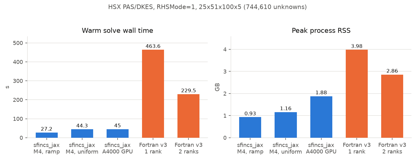
Measured warm solve time and peak process RSS. Regenerate with python tools/benchmarks/readme_figures.py; rerun the measurement with python tools/benchmarks/tier1_hsx_head_to_head.py.

Head-to-head (744k unknowns, HSX PAS DKES, RHSMode=1)

Configuration	Warm solve [s]	Peak RSS [GB]
dkx MacBook M4 CPU, Nxi-for-x ramp	27.2	0.93
dkx MacBook M4 CPU, uniform Nxi	44.3	1.16
dkx RTX A4000 GPU	45.0	1.88 (0.05 GB VRAM buffers)
SFINCS Fortran v3, 1 MPI rank	463.6	3.98
SFINCS Fortran v3, 2 MPI ranks (measured floor)	229.5	2.86

With the matched ramp discretization this is 17x faster than 1-rank Fortran and 8.4x faster than Fortran’s best measured parallel floor, at roughly 30% of the memory. Ramp-vs-uniform Nxi differences on the physics outputs are at most 0.9% (electrons). GPU time equals M4 CPU time because the Legendre scan is serial in L and the A4000 runs FP64 at 1/32 rate; GPU upside requires batching over (species, x, surfaces/Er) or fp32 factors with fp64 refinement. Scope: this is one measured 744k-unknown HSX PAS case; further cases are promoted as each vertical slice lands with its own evidence.

Fortran strong-scaling baseline (same case, same machine)

MPI ranks	Solve time [s]	Speedup	Parallel efficiency	Peak RSS [GB]
1	463.6	1.00	—	3.98
2	229.5	2.02	101%	2.86
4	240.9	1.92	48%	2.88
8	270.5	1.71	21%	1.61

Fortran/MUMPS saturates at 2 ranks on this machine and degrades beyond (performance/efficiency core asymmetry plus MUMPS OpenMP contention), so the practical Fortran floor for this case is about 230 s.

Cross-machine end-to-end time to solution

A second, independent sweep measures end-to-end wall time (operator build + solve + moments + output; run_profile on the dkx side, the full binary run on the Fortran side) for the two-species production variant of the same HSX PAS deck (1,275,010 unknowns) on two machines, with a freshly compiled Fortran v3 (conda PETSc 3.25 + MUMPS, MPI) and best-of-two repetitions per configuration. The Fortran run is one linear solve dominated by the preconditioner factorization plus a handful of Krylov applications, so end-to-end time is the honest cross-code metric. Reproduce with tools/benchmarks/time_to_solution.py.

Configuration	End-to-end [s]
Fortran MPI, 10-core laptop, n=1	350
Fortran MPI, 10-core laptop, best (n=8)	141
dkx, laptop, one process (cold / warm)	62 / 46
Fortran MPI, 36-core workstation, n=1	1163
Fortran MPI, 36-core workstation, best (n=8)	802
Fortran MPI, 36-core workstation, n=32	1423
dkx, workstation, one RTX A4000 GPU (cold / warm)	78 / 59
dkx, workstation, one CPU process (cold / warm)	6132 / 1998

The MPI scaling shape repeats on both machines: Fortran/MUMPS bottoms out around 8 ranks (1.4-2.5x over one rank) and degrades beyond — at 32 ranks the workstation run is slower than a single rank. One dkx process beats every measured Fortran configuration on the same hardware: 3.1x the laptop’s best MPI time on CPU, and 13.6x the workstation’s best MPI time on its GPU. The workstation’s CPU path is dominated by the serial Legendre scan at that machine’s low single-core throughput — on such hardware the GPU is the dkx backend of choice, and batched scans (dkx.batch, measured in tools/benchmarks/batched_scan.py) are the axis where one process replaces an entire MPI allocation.

Memory findings

• At the full production resolution of this case (Ntheta=25, Nzeta=115, Nxi=149, Nx=5; a 2,512,760-unknown system), neither code fits a global sparse factorization on a 24 GB machine: Fortran/MUMPS drove macOS swap to ~46.5 GB during factorization and was killed, and the dense/CSR JAX host paths are size-capped well below it.

• The truncated Legendre block elimination is the locally viable direct path: its memory is O(K m^2) with m = Ntheta * Nzeta (one ~66 MB 2875^2 block at production resolution, independent of Nxi). On the 744k case the truncated route needs ~0.3 GB where a full-band tier-1 factor would need ~91 GB.

Solver-noise finding

The direct solve is more converged than the Fortran reference: Fortran’s own electron FSABFlow scatters 51% across its 1/2/4/8-rank runs of this case (KSP rtol=1e-6 iterative-solver noise), while dkx matches the closest Fortran run to 2e-10 and sits inside Fortran’s own spread on every compared quantity.

Parity referees

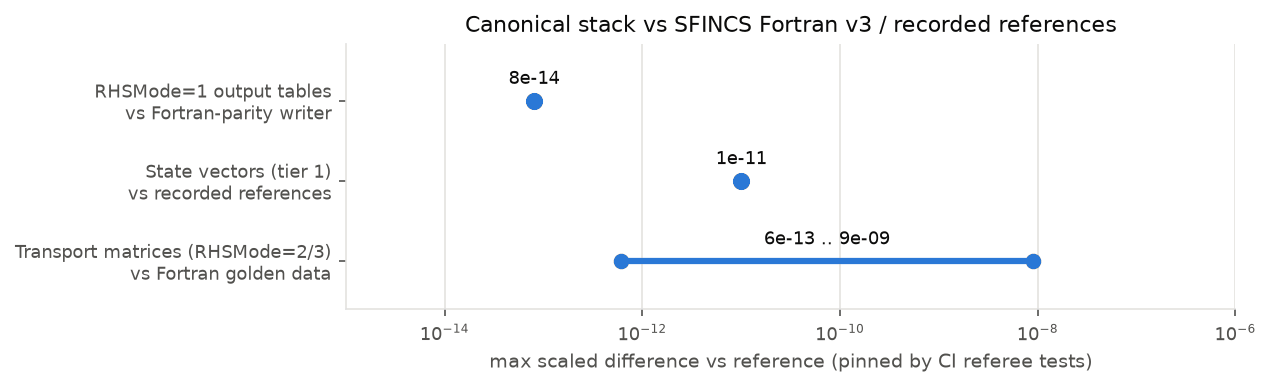
Parity envelopes pinned by the CI referee tests (tests/test_run_rhsmode1.py, tests/test_run_transport.py): RHSMode=1 output tables at 8e-14, tier-1 state vectors vs recorded references at 1e-11, RHSMode=2/3 transport matrices vs Fortran golden data at 6e-13 .. 9e-9.

Known issues

• Silently wrong tier-2 adjoint on singular FP systems. Full Fokker-Planck with constraintScheme=1 on the flagship-optimization deck yields a numerically singular system (~5 zero singular values, condition number ~2e36); the tier-2 GCROT adjoint stagnates and the implicit-diff VJP returns a wrong gradient without any error (AD -1.7e-3 vs FD +2.8e-5 on the affected dof). PAS+``Er`` tier-2 gradients on the same chain are exact (2.9e-6 vs FD). Fix direction: surface adjoint-solve convergence in SolveResult and raise/flag when the adjoint residual misses tolerance. A reproducer is tracked.

• Ill-conditioned scheme-1 monoenergetic off-diagonal. The Fortran build itself fails upstream’s tests.py on the monoenergetic_geometryScheme1 transportMatrix[0,1] element only (+1.62 vs expected -1.08 at solverTolerance=1e-6; +26.3 at 1e-12 — tolerance-unstable, so the element is ill-conditioned in this configuration). Parity tests pin that element to upstream’s expected value (-1.07986), which the dkx direct solve reproduces to 4.2e-6.

CPU and GPU: where each wins

The structured tier-1 path is the one that lets dkx fit and finish a production case; the honest headline is that a development-MacBook CPU and a workstation RTX A4000 land at parity on the direct tier, while the iterative and small-system paths favored the MacBook CPU — note these two backends live on different machines; the same-host CPU-vs-GPU picture is measured in “Same-host CPU/GPU crossover” below and looks very different. The full 744k-unknown HSX case was re-measured on both backends after the ramp-aware truncated kernel became the canonical route:

Post-fix 744k HSX PAS/DKES head-to-head (end-to-end = build + solve)

Backend	Runtime	Peak RSS
SFINCS Fortran v3 (PETSc + MUMPS, dev MacBook)	> 2.6 h, unfinished	3.6-5.7 GB
dkx CPU (dev MacBook)	41.4 s e2e (25.0 s warm solve)	1.35 GB
dkx GPU (RTX A4000)	59.6 s e2e (26.2 s warm solve)	2.3 GB

Both machines route block_tridiagonal_truncated and land within a few seconds of each other on the warm solve; under the tier-2 recycled-Krylov route the same case ran out of memory on the 16 GB GPU, so the structured tier is what makes it fit at all. A mid-size HSX case (336k unknowns) is at MacBook-CPU-vs-A4000 parity as well (3.5 s versus 3.3 s warm).

The GPU does not help the iterative and small-system paths relative to a fast development CPU. Full Fokker-Planck GCROT, the \(\Phi_1\) Newton solve, value_and_grad, the ambipolar Brent root, and a one-shot monoenergetic solve all ran 2-5x slower on the A4000 than on the development MacBook’s CPU. A dedicated same-host re-measurement (next section) showed that this comparison mixes machines: on the workstation that hosts the A4000, the GPU beats that machine’s own 36-core CPU on essentially every path and size, and the tier-1 production solve is FP64-compute-bound on the card (1/32-rate FP64), not dispatch-bound. The honest summary is per-machine: a fast laptop CPU beats a modest workstation GPU on small and iterative work; on the GPU’s own host the GPU wins, and batched work — multi-\(E_r\) or multi-surface vmap sweeps — widens that win.

Same-host CPU/GPU crossover (2026-07)

All numbers in this section come from one host (36-core Pop!_OS workstation, RTX A4000 16 GB, JAX 0.10.2, CUDA_VISIBLE_DEVICES=0), so CPU and GPU columns are the clean comparison; the development-MacBook CPU column is included to expose the cross-machine effect. Warm = second identical solve() in-process (cached executable); cold = first solve in a fresh process with a populated persistent compilation cache. Reproduce with tools/benchmarks/gpu_cpu_ladder.py.

Tier-1 (direct truncated block-Thomas, the production route) — the GPU won every measured size, 2.7x to 39x, so there is no same-host CPU/GPU crossover above the smallest deck measured (6.5k unknowns):

Warm tier-1 solve, HSX PAS/DKES family (seconds)

Unknowns	Workstation CPU	Workstation GPU	Dev-MacBook CPU (other machine)
6,488	1.41	0.53	—
40,584	3.04	1.17-2.20	0.62-0.73
78,010	6.32	1.48	—
224,410	45.4	2.49	—
336,610	20.8-33.1	2.97-3.70	1.81
688,810	—	9.35	—
1,275,010 (production deck)	1,036	26.0-26.5	—

The production point is the full 2-species HSX deck (25x51x100x5 = 1,275,010 unknowns): workstation CPU end-to-end 2,000.6 s (build 8.8 s, cold solve 952 s, warm solve 1,036 s) versus GPU end-to-end 72 s (warm solve 26.0 s) — a 39x same-host GPU win. Two honesty notes: the workstation CPU warm repeat measured slower than its cold solve (1,036 s vs 952 s) and the 224k/336k rungs overlap (45.4 s vs 20.8-33.1 s), i.e. all-core CPU timings on this box carry large run-to-run variance (thermal steady state at ~34-thread load); and the earlier “~1,998 s office CPU warm” figure matches this end-to-end total, not the warm solve alone.

Tier-2 (GCROT-recycled FGMRES, preconditioned) — the GPU also won every measured size warm; again no same-host crossover down to the smallest practical Fokker-Planck deck:

Warm tier-2 GCROT solve, W7-X FP family (seconds)

Unknowns	Workstation CPU	Workstation GPU	GPU speedup
2,804	1.38	0.93	1.5x
11,884	4.03	2.75	1.5x
78,628	21.7	12.0	1.8x
155,524	67.8	25.2	2.7x

Cold-including-compile favors the CPU at the small end (2.8k: 21.0 s CPU vs 24.3 s GPU; 11.9k: 19.2 s vs 28.5 s) because GPU compilation is slower — a first-run effect the persistent cache removes on repetition.

Iterative and small-system paths, same host — value_and_grad through the tier-1 solve (39.3k unknowns): warm 4.21 s CPU vs 3.03 s GPU; the ambipolar Brent root (2 species): 92.8 s CPU vs 48.4 s GPU end-to-end. The single measured CPU-wins case is the \(\Phi_1\) Newton solve, whose unpreconditioned inner GCROT systems are capped at 6,000 unknowns (3,975 here): warm re-solve 0.048 s CPU vs 0.159 s GPU (2.6x) and cold 40.3 s vs 52.2 s. Per-solve() routing of just those inner solves to the CPU did not recover the win (0.12-0.13 s: the per-iteration Newton residuals stay on the GPU and each routed solve pays device transfers plus a one-time CPU compile), so small \(\Phi_1\)-heavy workloads are best run whole-process on the CPU (JAX_PLATFORMS=cpu).

Where the GPU time goes (profiler trace). A jax.profiler capture of the warm 336k tier-1 GPU solve records 31,953 kernel launches with a mean kernel duration of 0.086 ms; the device is busy 2.74 s of the 3.18 s device span (13.8% idle), and the untraced warm solve is 2.97 s — i.e. the tier-1 GPU solve is ~90% device compute, not host-dispatch-bound: the async dispatch pipeline keeps the serial Legendre scan’s small kernels queued ahead of execution. The top kernels are FP64 dense linear algebra — getrf (0.90 s), FP64 tensor-core GEMMs (0.80 s), trsm (0.45 s) — so the production solve sits within ~2.7x of the card’s FP64 arithmetic floor (~5.5 TFlop at ~0.6 TFLOPS FP64). Faster-FP64 hardware, not lower launch latency, is what would speed this path up.

Device routing knob. solve(device=...) gives explicit control: "cpu"/"gpu"/a jax.Device move the solve (inputs via jax.device_put, solution returned on the input’s device; inert under jit/grad tracing), and "auto" (default, env DKX_SOLVE_DEVICE) additionally consults the size thresholds DKX_SOLVE_CPU_MAX_SIZE_TIER1 / _TIER2. Both thresholds default to 0 — automatic CPU-routing disabled — because the measurements above do not support a nonzero default on the reference host; they exist for hosts where the CPU/GPU balance differs (e.g. a strong CPU next to a weak accelerator: set DKX_SOLVE_CPU_MAX_SIZE_TIER2=6000).

Cold starts and the persistent compilation cache. The cache configured by dkx.__init__ (default ~/.cache/dkx/jax_compilation_cache, min-compile-time and min-entry-size forced to 0, GPU per-fusion autotune cache on by JAX default) was audited working cross-process on this host: with a populated cache the small-deck GPU cold solve drops 10.8 s -> 1.7 s, the CPU cold solve 7.8 s -> 3.0 s, and the \(\Phi_1\) GPU cold solve 52.2 s -> 15.0 s; at the production size the CPU cold solve ran at warm speed (952 s vs 1,036 s warm). First-ever runs on a clean machine still pay full XLA compilation (historically ~2,100 s extra on the production CPU case), so cold -vs-warm expectations are: first run per (shape, backend) compiles; every later process reuses the cache and starts at warm speed plus a few seconds of cache loading.

Cyclic-reduction assessment (evaluation only, not adopted). Block cyclic reduction would replace the serial length-\(L\) block-Thomas recurrence with \(\log_2 L\) parallel levels, at 2-3x the arithmetic and a working set touching all \(L\) blocks per level. The trace above shows the regime it would need — a device idled by the serial scan — does not occur at production size: the A4000 is ~86% busy and FP64-throughput-bound, so inflating flops 2-3x to shorten the dependency chain would slow the solve down, and at small sizes (where the device is latency-bound) the absolute times are already sub-second and the memory-lean lax.map batching would have to be abandoned to expose the parallelism. Cyclic reduction only makes sense on hardware with FP64 headroom (data-center cards) combined with small \(N_\theta N_\zeta\) blocks and long \(L\) chains — the opposite corner from the production decks; it is left unimplemented.

Measured GPU anatomy and memory headroom (RTX A4000)

The same host quantifies how far the structured tier-1 route stretches a 16 GB card. All rows are warm best-of-N block_tridiagonal_truncated solves of HSX-family decks on the RTX A4000 (12.56 GB usable device budget), with the device peak read from jax device-memory statistics; every solve converged with residuals in 1e-13 .. 1e-15.

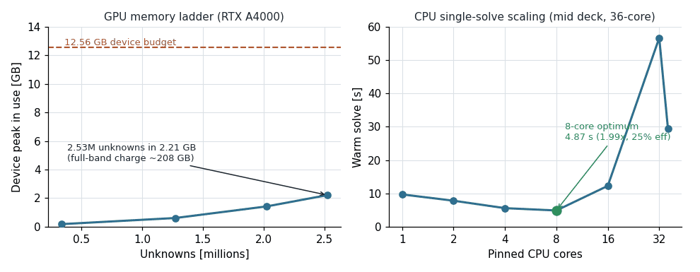
Left: single-GPU memory ladder — device peak stays far under the 12.56 GB budget, a 2.53M-unknown solve peaking at 2.21 GB. Right: 36-core CPU single-solve thread scaling on the mid deck (336,610 unknowns), warm solve versus pinned cores, bottoming at the 8-core optimum and inverting past it. Regenerate with python tools/benchmarks/gpu_anatomy_figure.py.

Warm tier-1 solve, single RTX A4000: memory ladder

Unknowns	Device peak [GB]	Warm solve [s]
336,610	0.18	3.7
1,275,010 (production)	0.61	25.6
2,025,010	1.42	85.3
2,525,010	2.21	157.6

The device peak grows far slower than the unknown count because the truncated tier-1 kernel only ever materializes its O(K m^2) working set (the lowest Legendre blocks), not the full band: the 2,525,010-unknown solve peaks at 2.21 GB where the conservative full-band charge for that system is ~208 GB, so multi-million-unknown decks fit with large headroom on the 16 GB card — the route-aware footprint model (End-to-end pipeline efficiency) is what lets the auto policy account for this truncated working set rather than the full-band peak. The first over-budget rung above 2,525,010 unknowns is the only measured out-of-memory point: its truncated working-set estimate is 26.25 GB, past the 12.56 GB device budget.

Per-phase anatomy for the production and mid decks (warm, same host):

Warm-solve phase breakdown [s]

Deck (unknowns)	Build	RHS	Warm solve	Moments
Mid (336,610)	2.85	1.55	3.7	3.78
Production (1,275,010)	6.36	2.74	25.6	5.57

The truncated solve dominates end-to-end time at the production size, while operator build, right-hand-side assembly, and moment evaluation stay a few seconds each. The device-memory budget knob (DKX_TIER1_MEMORY_BUDGET_GB) gates only batch chunking, not the single truncated solve: sweeping it across 2/8/32 on the mid deck leaves the warm solve at ~3.6-4.0 s and the device peak at ~0.12 GB in all three, confirming the single-solve footprint is budget-independent.

Production profiling battery

The per-case picture on CPU (development MacBook, idle, one fresh subprocess per case, via tools/benchmarks/profile_production.py):

Case	Unknowns	Method	Solve cold / warm	Peak RSS
HSX PAS/DKES, mid (ramp)	336,610	block_tridiagonal_truncated	4.1 s / 3.5 s	885 MB
W7-X full Fokker-Planck, 2 species	78,628	GCROT, 115 iters	17.5 s / 7.6 s	4.1 GB
Monoenergetic RHSMode=3, scheme 1	—	block_tridiagonal	4.8 s e2e	2.0 GB
PAS gradient (value_and_grad)	39,318	tier-1 differentiable	5.3 s / 2.1 s	4.3 GB
\(\Phi_1\) Newton	4,548	unpreconditioned GCROT	232 s / 0.04 s	1.4 GB
Ambipolar \(E_r\), 2 species	—	Brent root	31.2 s	3.9 GB

Two lessons stand out. First, promoting the ramp-aware truncated kernel into solve(method="auto") is what pulls the mid-size HSX case from the tier-2 route’s 10.8 GB / 15.4 s warm down to 885 MB / 3.5 s warm — 12x less memory and roughly 4x faster on the same deck, with the autodiff gradient through the ramped route still matching finite differences at rtol 1e-6. Second, the cold 232 s \(\Phi_1\) Newton solve (an unpreconditioned, restart-capped GCROT inner solve at only 4.5k unknowns) is the top remaining runtime target; its warm re-solve is already 0.04 s, so the cost is entirely first-call iteration count, not steady state.

Example-suite benchmark

A broader, fast-to-reproduce benchmark complements the single production case: it runs the full 39-case CPU/GPU example suite against SFINCS Fortran v3 and plots every row whose Fortran reference runtime clears a 10 s reference-runtime-window, so process launch, filesystem overhead, and JIT amortization do not dominate the shorter measurements. The full suite stays the parity audit; only the runtime/memory plot applies the window.

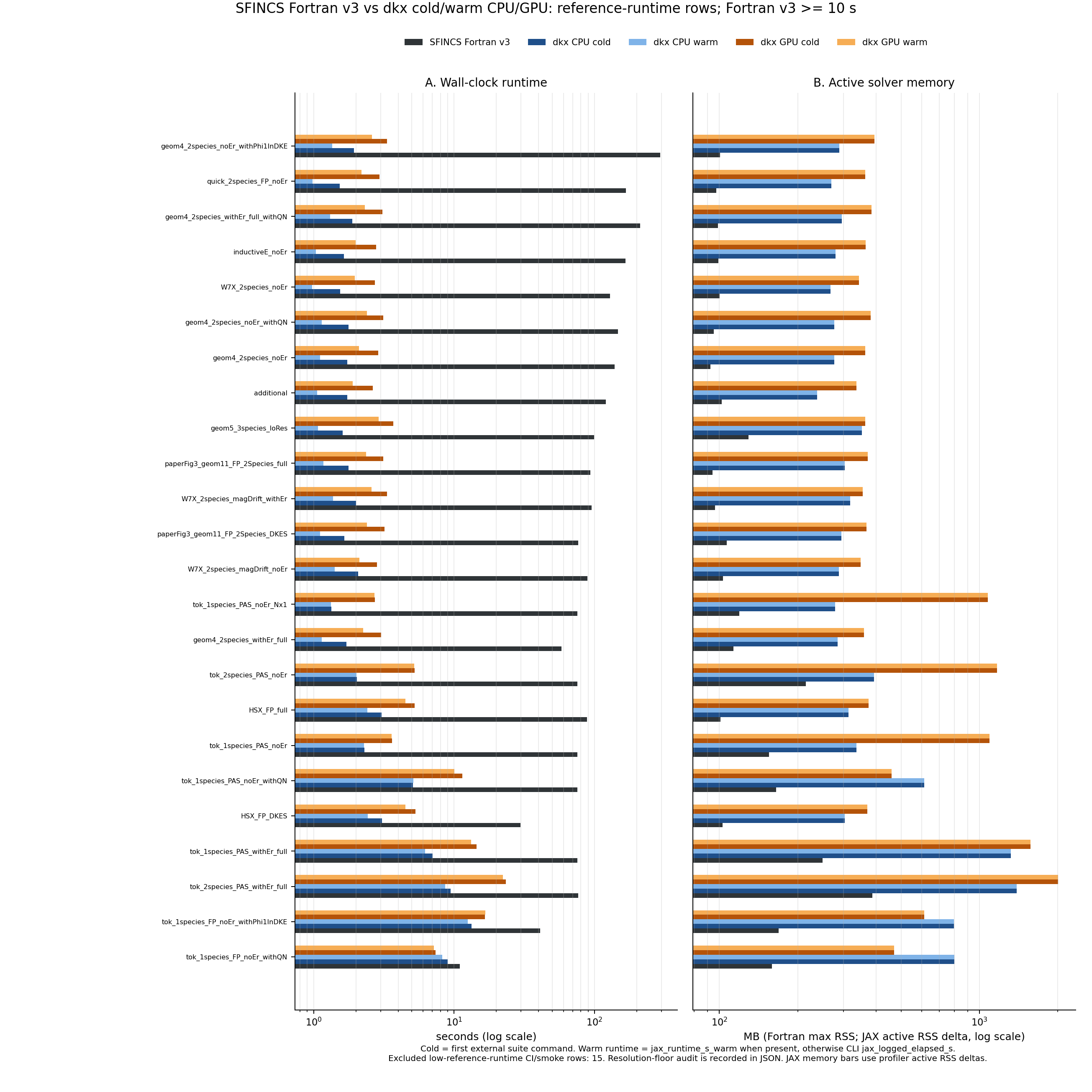
Example-suite benchmark. Runtime bars (left) and active-memory bars (right) for each reference-runtime-window case: SFINCS Fortran v3, dkx CPU cold/warm, and dkx GPU cold/warm, ordered by best warm dkx speedup over the Fortran v3 runtime. Fortran memory is process maximum RSS; JAX memory uses profiler RSS deltas over the fixed Python/JAX/XLA baseline. Reproduce with examples/publication_figures/generate_fortran_suite_benchmark_summary.py.

Across the plotted rows the median cold JAX/Fortran wall-clock ratio is about 0.021x on CPU and 0.037x on GPU. Median active-memory ratios are about 2.89x on CPU and 3.71x on GPU; the full process maximum-RSS ratios, kept in the summary JSON audit fields, are about 4.75x on CPU and 8.80x on GPU. The numeric summary and the top runtime/memory cases are recorded in examples/publication_figures/artifacts/dkx_fortran_suite_benchmark_summary.json.

Compile time vs steady state

JAX pays a one-time compile cost that a persistent cache amortizes across runs. The checked figure below separates the two for four reference transport cases: compile estimate (cold first call minus warm first call) versus steady warm solve time.

Per case, compile estimate = cold first call - warm first call; steady solve is the warm repeated runtime. Warm solves are tens of milliseconds once compiled, so repeated scans and optimization loops run at steady-state speed.

For steady-state benchmarking, take repeated JAX runs and report the warm timing; set a persistent JAX_COMPILATION_CACHE_DIR to reuse compiled kernels across processes.

End-to-end pipeline efficiency

The head-to-head figures above are warm solve times; a production run also parses the equilibrium, builds the operator, evaluates moments, and writes output. Three pipeline choices keep that wall-clock envelope small.

One build through every consumer. A run_profile(out_path=...) call threads a single KineticOperator build through the operator apply, the run-level geometry derivation, the two writer geometry-extras passes, and the moment evaluation, and dkx.magnetic_geometry.read_boozer_bc() memoizes each .bc parse on file identity. Building once, rather than re-parsing the 32 MB Boozer .bc per consumer, takes the warm end-to-end production run (the 1,275,010-unknown HSX PAS deck) from 43.6 s to 26.7 s, and the small reduced deck from 15.6 s to 2.3 s, with dataset-exact outputs on the six audited decks including the production case (a counting regression test in tests/test_run_rhsmode1.py pins the one-build behavior). Ambipolar loops, monoenergetic scans, and batched scans inherit the memoized parse for free.

Whole-file vectorized ``.bc`` parse. The Boozer .bc reader parses the whole file in one vectorized pass, bit-identical to the line-by-line reference it falls back to on ragged blocks. The 32 MB hsx3free.bc parses in 0.38 s against 2.22 s line-by-line (5.8x), and w7x_standardConfig.bc in 0.18 s against 1.34 s (7.3x); on the small deck the whole-file parse pulls the cold start from 6.19 s to 4.29 s and the operator build from 5.14 s to 2.58 s.

Route-aware memory footprint. The auto policy’s memory estimate models the kernel the solve actually executes. A deck that routes to the truncated tier-1 block-Thomas kernel is charged its truncated working set, not the full-band factorization peak that route never allocates. On the production deck that takes the estimate from 53.06 GB (the full-band charge) to 1.68 GB, against a measured process peak of ~1.16 GB; the mid deck drops from 6.16 GB to 0.73 GB. Charging the full-band peak had capped batched scans at a single chunk; the route-aware estimate un-serializes them. At a 19.2 GB budget the auto chunk count on the production deck rises from 1 to 11, and a mid-deck 8-point batched_er_scan runs in one chunk at 749 MB peak instead of three chunks at 2084 MB. The per-solve footprint model is dkx.solve.auto_solve_peak_memory_bytes(), which the batch chunker in dkx.batch reads to size its jax.lax.map chunks (Parallelism).

Performance patterns

The design choices that produce the numbers above, in one place:

• Matrix-free operators. The drift-kinetic Jacobian is applied as a pure function (tensor contractions and directional derivatives), never assembled as a sparse matrix, so it JIT-compiles for CPU/GPU and differentiates cleanly.

• Structured direct tier. The block-tridiagonal-in-\(L\) elimination with truncated storage is the memory lever: O(K m^2) with m = Ntheta*Nzeta, independent of Nxi (Numerics and algorithms).

• The \(N_\xi\)-for-\(x\) ramp. Fewer Legendre modes at high speed cut both work and memory; on the 744k HSX case the ramp is the difference between 0.93 GB and 1.16 GB at essentially identical physics outputs (\(\le 0.9\%\)).

• Subspace recycling. The tier-2 recycle pair warm-starts neighbouring points in an \(E_r\) scan or a \(\Phi_1\) Newton iteration, so continuation converges in a handful of iterations.

• Preconditioning by a simplified exact solve. Tier 2 is right-preconditioned by an exact tier-1 solve of a collision-/drift-simplified coarse operator (the Fortran preconditionerOptions idiom).

• Phi1-aware bordered-Schur coarse preconditioner. The \(\Phi_1\) Newton inner solve is preconditioned by a generalized bordered Schur complement that eliminates the quasineutrality border (the \(\Phi_1(\theta,\zeta)\) / \(\lambda\) / source rows) exactly through the coarse f-block solve plus a small dense Schur solve (dkx.solve.build_coarse_preconditioner()). On the production PAS Phi1 case this took the inner Krylov solve from 9198 unpreconditioned iterations (about 398 s) to 5 iterations (about 13.5 s), a roughly 29x speedup, with answers identical to machine precision and the differentiable path preserved.

• Short-recurrence Krylov for transport. RHSMode=2/3 solves default to memory-lean BiCGStab with a collision-diagonal preconditioner, with GMRES as a fallback.

• Gradient checkpointing. jax.checkpoint around collision operators and transport diagnostics trades recomputation for lower peak memory during autodiff on long chains.

• Build once, parse once. The run pipeline threads a single operator build through every consumer and memoizes .bc parses on file identity, and the .bc reader parses the whole file in one vectorized pass — the end-to-end and cold-start levers detailed under End-to-end pipeline efficiency.

• Route-aware memory estimate. The auto policy charges the truncated working set the solve actually allocates, not the full-band factorization peak, which un-serializes batched scans into memory-budgeted chunks (End-to-end pipeline efficiency and Parallelism).

For the equations and derivations behind these techniques, see Numerics and algorithms and Differentiability; for parallel-execution knobs and batched scans, see Parallelism.

Differentiable paths

Gradients are exact and cost about one extra solve, because the adjoint reuses the forward factorization through the implicit function theorem. What is differentiable (geometry, profiles, the ambipolar \(E_r\), the \(\Phi_1\) state, the monoenergetic transport matrix), the measured gradient-vs-finite- difference agreement, and the honest tier-2 singular-Fokker-Planck caveat are all documented in Differentiability.