Optimization Workflows
dkx supports optimization workflows in two layers:
Fast differentiable proxies used inside a stellarator optimizer.
High-fidelity kinetic gates run on accepted designs before making a physics or publication claim.
This split is deliberate. A full neoclassical solve at every VMEC objective
evaluation is usually too expensive, and it can make optimizer behavior depend
on solver tolerances, branch choices, and one-off failed scans. The recommended
workflow is therefore to optimize with cheap JAX-native terms and promote only
selected candidates to full dkx scans.
The implementation lives in
dkx.workflows.optimization and the public example is
examples/optimization/qa_nfp2_dkx_objectives.py.
QA nfp=2 Example
Run the fast QA optimization lane from the repository root:
python examples/optimization/qa_nfp2_dkx_objectives.py \
  --objective balanced \
  --steps 120 \
  --out-dir docs/_static/figures/optimization \
  --stem qa_nfp2_dkx_optimization_lane
This produces a JSON provenance file plus PNG/PDF figures:
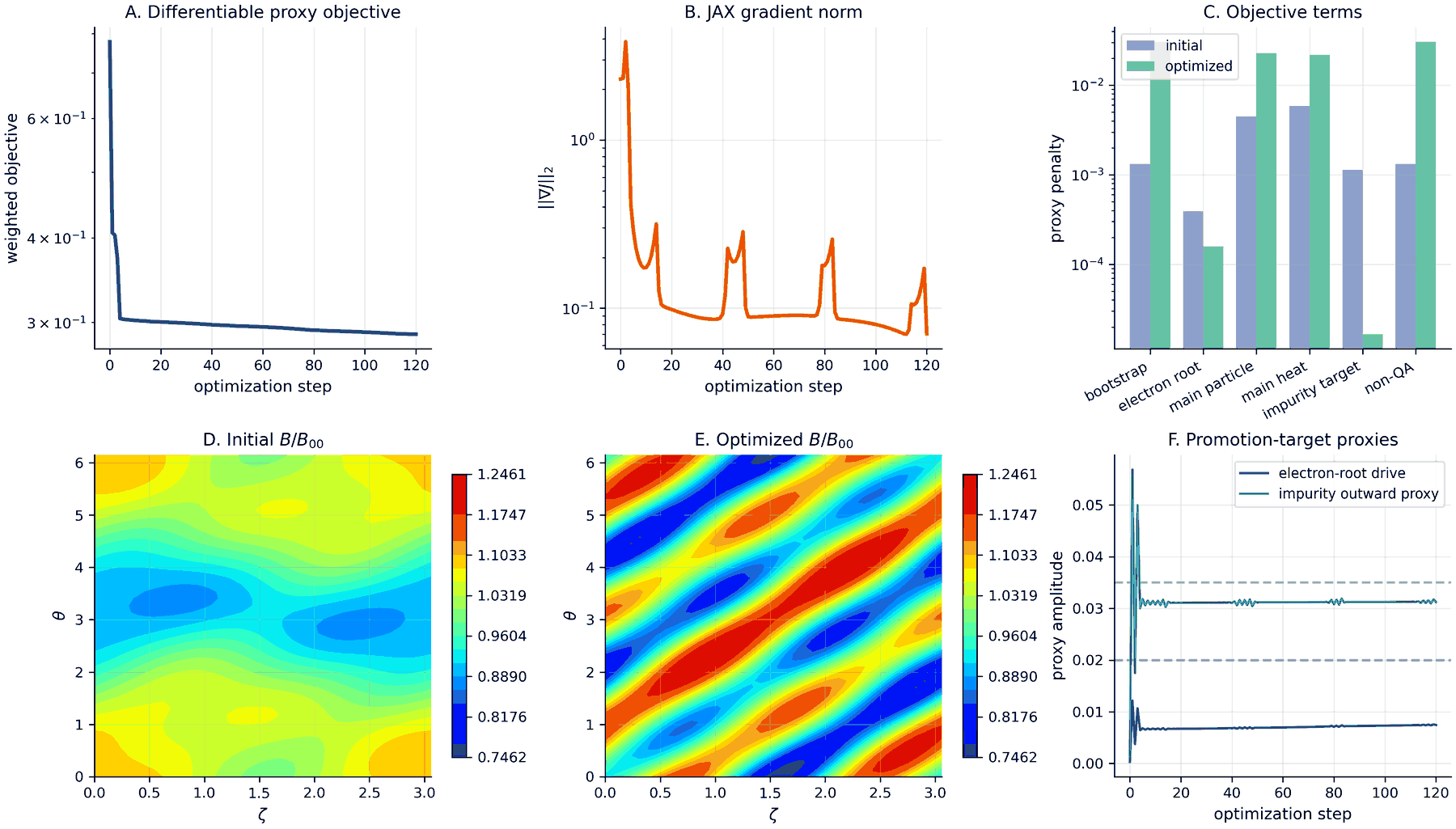
Fast QA nfp=2 neoclassical optimization proxy. Panels A-B show the differentiable JAX objective and gradient norm. Panel C shows the proxy terms before and after optimization. Panels D-E show the initial and optimized normalized Boozer field strength. Panel F shows the proxy electron-root and impurity-flux target amplitudes. This figure is an optimizer-design diagnostic, not a replacement for high-fidelity SFINCS kinetic validation.
Available objective presets are:
bootstrapPrioritize small bootstrap-current and QA-like geometry penalties.
electron-rootPrioritize a proxy for a resolved positive ambipolar root.
flux-selectivePenalize main-species heat and particle flux while encouraging outward impurity flux.
balancedCombine all terms in one tradeoff objective for demonstrations and optimizer smoke tests.
Bootstrap-Current Comparison Example
The most direct way to teach the geometry-to-transport workflow is to start from
the real vmex QA optimization output, verify that the VMEC equilibrium
has the intended finite rotational transform, and then use that equilibrium as
the input to kinetic dkx promotion scans. The checked figure below
uses vmex/examples/optimization/QA_optimization.py, whose public target
is aspect ratio 5 and mean iota 0.41.
python examples/optimization/qa_nfp2_bootstrap_current_comparison.py \
  --vmex-root /path/to/vmex \
  --out-dir docs/_static/figures/optimization \
  --stem qa_nfp2_bootstrap_current_comparison

VMEC-backed QA nfp=2 optimization diagnostic. Panels A-B show the real
VMEC last-closed-flux-surface and LCFS field strength. Panel C shows LCFS
cuts. Panel D shows the finite rotational-transform profile from the final
VMEC wout. Panel E shows the VMEC equilibrium current diagnostic
\(J\cdot B/\sqrt{B\cdot B}\) versus normalized toroidal-flux radius.
Panel F audits the QA_optimization.py objective and the final aspect/iota
gate. The checked artifact has aspect ratio 4.999999 and mean iota 0.4097.
Pass --comparison-result-dir to overlay a second vmex result, for
example a QA run in which QA_optimization.py has been edited to add
JDotB or RedlBootstrapMismatch to objective_tuples. That overlay is
accepted only if it reduces the VMEC current diagnostic while preserving the
finite-iota/aspect gate. The plotted current profile is still not a completed
kinetic SFINCS current. A candidate selected from this step should be promoted
with completed dkx scan-er outputs. The corresponding kinetic
observable is FSABjHatOverRootFSAB2,
which should be checked together with residual convergence, CPU/GPU agreement, radial and velocity-space convergence, and SFINCS Fortran v3 comparison when the input lies in shared model scope.
For a directly editable script, use
examples/optimization/QA_optimization_bootstrap_current.py. It follows the
same workflow as vmex/examples/optimization/QA_optimization.py but sets
MAX_MODE = 3 for faster iteration and exposes
INCLUDE_BOOTSTRAP_CURRENT_OBJECTIVE at the top of the file. Run once with
the flag disabled, once with it enabled, then compare the two result
directories:
DKX_VMEX_ROOT=/path/to/vmex \
  python examples/optimization/QA_optimization_bootstrap_current.py

python examples/optimization/qa_nfp2_bootstrap_current_comparison.py \
  --vmex-root /path/to/vmex \
  --qa-result-dir results/qa_opt_bootstrap_current_maxmode3/qa_only \
  --comparison-result-dir results/qa_opt_bootstrap_current_maxmode3/with_jdotb_current_objective
Objective Terms
Bootstrap current
For a set of radial surfaces \(\rho_i\), the high-fidelity bootstrap-current objective is
In dkx output this uses FSABjHatOverRootFSAB2. The helper
bootstrap_current_objective evaluates the normalized least-squares penalty
from completed kinetic outputs or cached radial profiles.
Ambipolar electron root
The radial current used for ambipolarity is
where \(\Gamma_s\) is the radial particle flux for species \(s\). An electron-root objective requires a resolved positive root
The helper find_ambipolar_roots sorts the scan, finds bracketed roots, and
classifies each root as ion, near-zero, or electron. The helper
electron_root_penalty returns zero only when a positive root exists with a
finite local slope. This avoids promoting flat or unbracketed ambipolar curves
as meaningful electron-root evidence.
Flux selectivity
For main species \(m\) and an impurity species \(Z\), the selected flux objective is
The last term is written as a shortfall penalty rather than an unbounded
maximize impurity flux objective. This keeps the optimizer well-scaled and
prevents it from increasing impurity transport at any cost.
Differentiable Proxy
The public proxy path uses a Boozer spectrum
with the \(B_{00}\) component fixed. For QA optimization, terms with \(n_k \ne 0\) are treated as non-QA content. The differentiable proxy combines field-strength variance, angular roughness, non-QA spectral energy, and smooth hinge penalties for electron-root and impurity-flux targets.
The proxy layer is evaluated with JAX and checked by finite differences through
qa_proxy_gradient_gate. It is appropriate for optimizer steering, unit
tests, and rapid design iteration. It is not a high-fidelity kinetic transport
claim, and it does not make the later promoted kinetic scan-er outputs
differentiable.
High-Fidelity Promotion Gates
Accepted designs should be promoted to actual dkx solves before
publication or engineering decisions. Real promotion starts only after the
candidate has completed dkx scan-er outputs containing
sfincsOutput.h5 files for the requested electric-field grid. The minimum
promotion evidence is:
Same-profile
dkxelectric-field scans over each selected radius.Ambipolar root bracketing with a positive electron root when requested.
Bootstrap-current normalization audit using
FSABjHatOverRootFSAB2.Particle, heat, and impurity flux sign-convention audit.
Linear residual convergence and solver-path provenance.
CPU/GPU agreement for selected final designs.
SFINCS Fortran v3 comparison when the case lies in the shared model scope.
The helper kinetic_validation_gate records residual and CPU/GPU agreement
checks for promoted designs. For production optimization campaigns, store the
JSON summary generated by each proxy run together with the completed SFINCS
scan outputs and solver traces. The synthetic scan generated when
evaluate_dkx_promotion_scan.py is run without --scan-dir is only
a plotting/API demonstration and must not be treated as promotion evidence.
Real Promotion Checklist
Replace the paths and electric-field grid with the accepted candidate’s actual
VMEC geometry, profiles, species, radial surface, and campaign tolerances. The
promotion boundary is the first command that evaluates a completed scan-er
directory; anything before that is proxy provenance or scan planning.
mkdir -p runs/qa_candidate01/proxy runs/qa_candidate01/audit
python examples/optimization/qa_nfp2_dkx_objectives.py \
  --objective balanced \
  --steps 120 \
  --out-dir runs/qa_candidate01/proxy \
  --stem candidate01_proxy
python examples/optimization/launch_dkx_candidate_scan.py \
  --proxy-summary runs/qa_candidate01/proxy/candidate01_proxy.json \
  --input runs/qa_candidate01/input_r0p50.namelist \
  --out-dir runs/qa_candidate01/scan_cpu/r0p50 \
  --er-min -3 \
  --er-max 3 \
  --n-er 7 \
  --jobs 4 \
  --impurity-species-index 2 \
  --target-impurity-flux 0.01
Run production evidence as explicit scan, audit, and comparison commands. This keeps the stable examples small and makes each expensive CPU, GPU, or optional Fortran-v3 lane scheduler-friendly. Fortran-v3 HDF5 files often do not contain the JAX linear-residual datasets, so only relax residual requirements for Fortran-derived promotion JSON files when that absence is documented.
JAX_PLATFORM_NAME=cpu dkx scan-er \
  --input runs/qa_candidate01/input_r0p50.namelist \
  --out-dir runs/qa_candidate01/scan_cpu/r0p50 \
  --values -3 -2 -1 0 1 2 3 \
  --compute-solution \
  --skip-existing \
  --jobs 4
python examples/optimization/evaluate_dkx_promotion_scan.py \
  --scan-dir runs/qa_candidate01/scan_cpu/r0p50 \
  --out-dir runs/qa_candidate01/audit \
  --stem candidate01_r0p50_cpu \
  --require-electron-root \
  --impurity-species-index 2 \
  --target-impurity-flux 0.01
CUDA_VISIBLE_DEVICES=0 JAX_PLATFORM_NAME=gpu dkx scan-er \
  --input runs/qa_candidate01/input_r0p50.namelist \
  --out-dir runs/qa_candidate01/scan_gpu/r0p50 \
  --values -3 -2 -1 0 1 2 3 \
  --compute-solution \
  --skip-existing \
  --jobs 1
python examples/optimization/evaluate_dkx_promotion_scan.py \
  --scan-dir runs/qa_candidate01/scan_gpu/r0p50 \
  --out-dir runs/qa_candidate01/audit \
  --stem candidate01_r0p50_gpu \
  --require-electron-root \
  --impurity-species-index 2 \
  --target-impurity-flux 0.01
python examples/optimization/compare_dkx_promotion_runs.py \
  --cpu runs/qa_candidate01/audit/candidate01_r0p50_cpu.json \
  --gpu runs/qa_candidate01/audit/candidate01_r0p50_gpu.json \
  --out-dir runs/qa_candidate01/audit \
  --stem candidate01_r0p50_comparison
If the case is in shared SFINCS Fortran v3 scope, add a Fortran-derived scan audit before the final comparison:
for run_dir in runs/qa_candidate01/scan_cpu/r0p50/Er*; do
  er_dir=$(basename "${run_dir}")
  mkdir -p "runs/qa_candidate01/scan_fortran/r0p50/${er_dir}"
  dkx run-fortran \
    --exe /path/to/sfincs \
    --input "${run_dir}/input.namelist" \
    --workdir "runs/qa_candidate01/scan_fortran/r0p50/${er_dir}"
done
python examples/optimization/evaluate_dkx_promotion_scan.py \
  --scan-dir runs/qa_candidate01/scan_fortran/r0p50 \
  --out-dir runs/qa_candidate01/audit \
  --stem candidate01_r0p50_fortran \
  --require-electron-root \
  --impurity-species-index 2 \
  --target-impurity-flux 0.01
python examples/optimization/compare_dkx_promotion_runs.py \
  --cpu runs/qa_candidate01/audit/candidate01_r0p50_cpu.json \
  --gpu runs/qa_candidate01/audit/candidate01_r0p50_gpu.json \
  --fortran runs/qa_candidate01/audit/candidate01_r0p50_fortran.json \
  --out-dir runs/qa_candidate01/audit \
  --stem candidate01_r0p50_comparison
Promotion Scan Example
After running an electric-field scan for an accepted candidate, evaluate it with:
python examples/optimization/evaluate_dkx_promotion_scan.py \
  --scan-dir /path/to/completed/scan-er-directory \
  --out-dir promotion_audit \
  --stem candidate01_promotion
The script reads each completed sfincsOutput.h5 file, computes
\(\sum_s Z_s\Gamma_s(E_r)\), classifies ambipolar roots, audits bootstrap
current and species fluxes, and checks linear residual diagnostics. If
--scan-dir is omitted, it creates a tiny synthetic SFINCS-style scan so the
plotting and gate logic can be demonstrated without a long solve. That
synthetic mode is demo-only and cannot promote an optimization candidate.
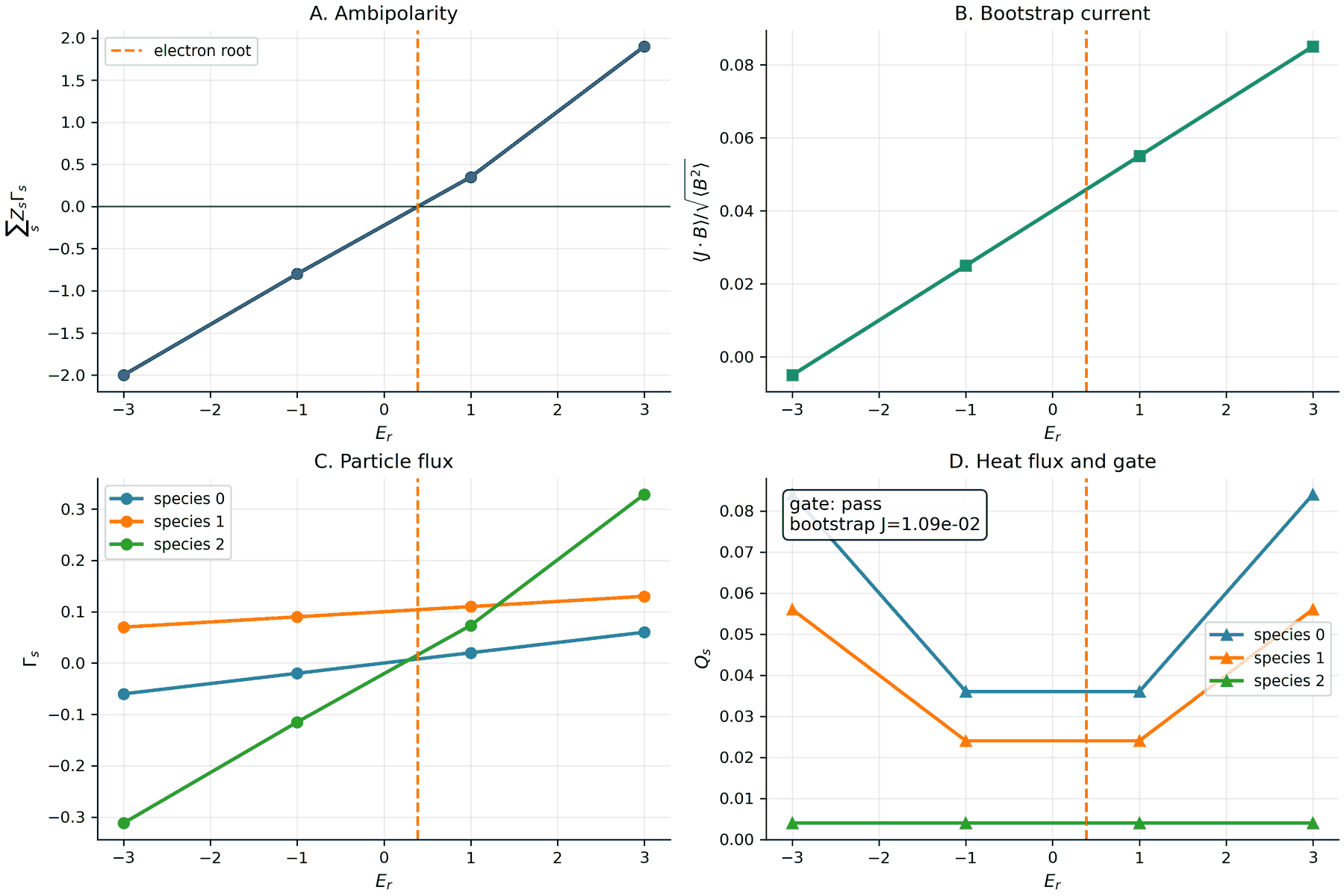
Promotion dashboard for an optimization candidate. Panel A shows the
ambipolar radial-current bracket and selected electron root. Panel B shows
the bootstrap-current observable. Panels C-D show particle and heat fluxes
by species, together with the promotion gate status. Real optimization
campaigns should use completed dkx scan-er outputs rather than the
synthetic demonstration scan used to generate this documentation artifact.
Practical End-To-End Lane
Use this lane when a QA optimizer has produced a small set of accepted
vmex candidates and you want a reproducible path from proxy evidence to
kinetic validation. The repository does not make vmex or
booz_xform_jax hard dependencies; a production campaign may run the VMEC
optimization in a separate checkout and hand this repository an accepted
wout plus the SFINCS profiles, species, radial surface, and resolution.
The scalar optimized in the proxy stage has the same role as the terms above:
Here \(\mathbf{a}\) are the active Boozer-spectrum coefficients and \(\widehat B = B/B_{00}\). This objective is an optimizer-steering scalar, not a kinetic solve. It can rank candidates and record a gradient/provenance gate, but it cannot by itself establish ambipolar roots, bootstrap-current accuracy, flux sign conventions, CPU/GPU agreement, or Fortran parity.
Run the optional VMEC/Boozer preflight and proxy-gradient workflow.
The status command is safe when optional geometry packages are absent:
python examples/optimization/vmex_workflow_status.py --json
For an accepted
vmexcandidate with a writtenwoutfile, persist the file-backed proxy-gradient provenance:mkdir -p runs/qa_candidate01/proxy python examples/autodiff/vmex_to_boozer_sfincs_pipeline.py \ --wout /path/to/vmex/run/wout_candidate01.nc \ --mboz 3 \ --nboz 3 \ --surface 0.5 \ --steps 0 \ --summary-json runs/qa_candidate01/proxy/vmec_boozer_proxy_gradient.json
For the repository-local QA nfp=2 proxy smoke test, run:
python examples/optimization/qa_nfp2_dkx_objectives.py \
  --objective balanced \
  --steps 120 \
  --out-dir runs/qa_candidate01/proxy \
  --stem candidate01_proxy
The resulting
candidate01_proxy.jsonis provenance for the proxy objective, not a SFINCS input file. It should travel with the accepted candidate so later audits can see the weights, final proxy coefficients, finite-difference gradient gate, and required promotion plan.Build the SFINCS input and run the high-fidelity electric-field scan.
Create a normal SFINCS
input.namelistfor the accepted VMEC geometry and selected radial surface. The input must encode the same profiles and species used for the physics claim. To create an auditable scan plan without starting a long run, use:python examples/optimization/launch_dkx_candidate_scan.py \ --proxy-summary runs/qa_candidate01/proxy/candidate01_proxy.json \ --input runs/qa_candidate01/input_r0p50.namelist \ --out-dir runs/qa_candidate01/scan_cpu/r0p50 \ --er-min -3 \ --er-max 3 \ --n-er 7 \ --jobs 4 \ --impurity-species-index 2 \ --target-impurity-flux 0.01
This writes
candidate_scan_plan.jsonwith the exactscan-ercommand and the follow-up promotion-audit command. Add--executeonly when you are ready to launch the scan. The equivalent direct command is:mkdir -p runs/qa_candidate01/scan_cpu/r0p50 JAX_PLATFORM_NAME=cpu dkx scan-er \ --input runs/qa_candidate01/input_r0p50.namelist \ --out-dir runs/qa_candidate01/scan_cpu/r0p50 \ --values -3 -2 -1 0 1 2 3 \ --compute-solution \ --skip-existing \ --jobs 4
For
RHSMode=2orRHSMode=3transport-matrix inputs, use--compute-transport-matrixinstead of--compute-solution:JAX_PLATFORM_NAME=cpu dkx scan-er \ --input runs/qa_candidate01/input_r0p50.namelist \ --out-dir runs/qa_candidate01/scan_cpu/r0p50 \ --min -3 \ --max 3 \ --n 13 \ --compute-transport-matrix \ --skip-existing \ --jobs 4
The scan directory contains subdirectories such as
Er1/andEr-1/. Each completed point must containsfincsOutput.h5. The ambipolar curve audited downstream is\[j_r(E_r) = \sum_s Z_s\Gamma_s(E_r), \qquad j_r(E_r^\star)=0 .\]A claimed electron root additionally needs \(E_r^\star>0\) and a bracketed sign change with finite local slope.
Audit the promoted scan.
The promotion audit reads the completed scan outputs, computes the ambipolar roots, checks bootstrap-current and flux observables, and records residual diagnostics:
python examples/optimization/evaluate_dkx_promotion_scan.py \
  --scan-dir runs/qa_candidate01/scan_cpu/r0p50 \
  --out-dir runs/qa_candidate01/audit \
  --stem candidate01_r0p50_cpu \
  --require-electron-root
If you also want upstream-style ambipolar root files in the scan directory, run:
dkx ambipolar-solve \
  --scan-dir runs/qa_candidate01/scan_cpu/r0p50 \
  --n-fine 1000
For
RHSMode=1inputs where the root should be solved directly instead of inferred from a precomputed scan, use the in-process Brent driver:dkx ambipolar \ --input runs/qa_candidate01/input_r0p50.namelist \ --out-dir runs/qa_candidate01/ambipolar_cpu/r0p50 \ --er-min -3 --er-max 3 --er-initial 0
This direct path writes per-evaluation
sfincsOutput.h5files and solver traces, then summarizes the selected solver lane, residual, timing, active size, cache provenance, and shape-checked Krylov state reuse inambipolar_result.json.Passing this audit means the specific completed scan has internally consistent promotion evidence. It does not imply convergence with respect to kinetic resolution, radial grid choice, profile uncertainty, or optimizer robustness unless those studies are run and stored separately.
Compare CPU, GPU, and Fortran evidence at selected final points.
Re-run the same scan on a GPU-capable installation:
mkdir -p runs/qa_candidate01/scan_gpu/r0p50
CUDA_VISIBLE_DEVICES=0 JAX_PLATFORM_NAME=gpu dkx scan-er \
  --input runs/qa_candidate01/input_r0p50.namelist \
  --out-dir runs/qa_candidate01/scan_gpu/r0p50 \
  --values -3 -2 -1 0 1 2 3 \
  --compute-solution \
  --skip-existing \
  --jobs 1
Compare matching CPU/GPU scan points near the selected ambipolar root:
ER_DIR=Er1
dkx compare-h5 \
  --a runs/qa_candidate01/scan_cpu/r0p50/${ER_DIR}/sfincsOutput.h5 \
  --b runs/qa_candidate01/scan_gpu/r0p50/${ER_DIR}/sfincsOutput.h5 \
  --rtol 1e-8 \
  --atol 1e-10 \
  --show-all
When the case lies in the shared
dkx/SFINCS Fortran v3 model scope and a compiled Fortran executable is available, run the same selected point through Fortran and compare the HDF5 outputs:mkdir -p runs/qa_candidate01/fortran/r0p50_${ER_DIR} dkx run-fortran \ --input runs/qa_candidate01/scan_cpu/r0p50/${ER_DIR}/input.namelist \ --workdir runs/qa_candidate01/fortran/r0p50_${ER_DIR} dkx compare-h5 \ --a runs/qa_candidate01/scan_cpu/r0p50/${ER_DIR}/sfincsOutput.h5 \ --b runs/qa_candidate01/fortran/r0p50_${ER_DIR}/sfincsOutput.h5 \ --rtol 1e-8 \ --atol 1e-10 \ --show-all
A compact way to describe the numerical comparison is
\[\delta_y(A,B) = \frac{\|y_A-y_B\|_\infty} {\max(\|y_B\|_\infty, y_\mathrm{floor})}.\]Set the actual tolerances in the campaign record before looking at the results, and keep them observable-specific. CPU/GPU agreement establishes backend reproducibility for the compared inputs. Fortran agreement establishes reference parity only for keys and physics options supported by both implementations. Neither comparison upgrades a proxy-only candidate to a publication claim unless the promoted kinetic scans, convergence evidence, and claim-specific tolerances are all archived.
Once the CPU, GPU, and optional Fortran promotion JSON files exist, create a compact comparison report:
python examples/optimization/compare_dkx_promotion_runs.py \
  --cpu runs/qa_candidate01/audit/candidate01_r0p50_cpu.json \
  --gpu runs/qa_candidate01/audit/candidate01_r0p50_gpu.json \
  --fortran runs/qa_candidate01/audit/candidate01_r0p50_fortran.json \
  --out-dir runs/qa_candidate01/audit \
  --stem candidate01_r0p50_comparison
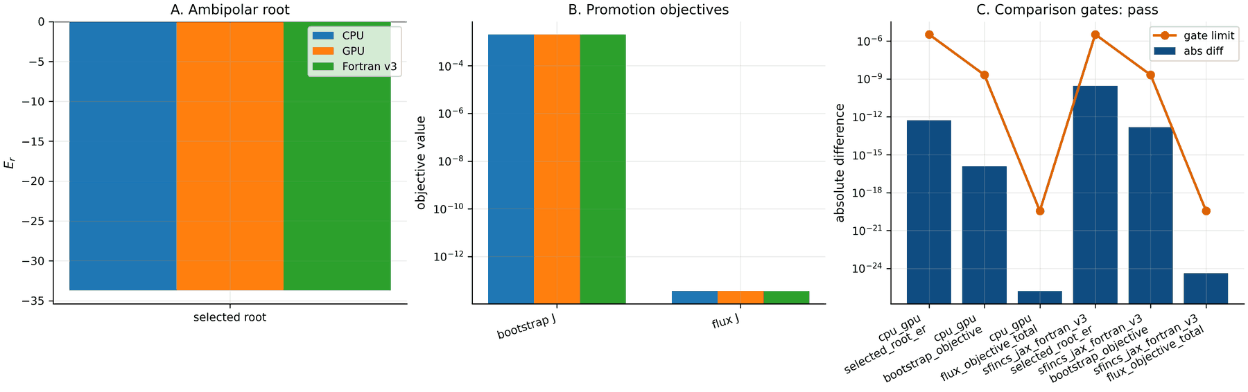
Real reduced-W7-X promotion comparison generated from separate completed CPU, GPU, and SFINCS Fortran v3 promotion JSON files. The scan used the shared PAS/DKES two-species model scope with \(N_\theta=7\), \(N_\zeta=11\), \(N_\xi=10\), and \(N_x=4\). The selected root is an ion root, \(E_r=-33.714544096\), so this artifact validates backend/reference agreement for the promotion machinery and shared model outputs; it is not an electron-root or finite-beta QA optimization claim.
The reduced-W7-X comparison passed the default strict gates without relaxed tolerances: CPU/GPU root, bootstrap-objective, and flux-objective relative differences were below \(5\times 10^{-13}\), and the DKX versus Fortran-v3 differences were below \(8\times 10^{-11}\). The checked demo/format-only comparison remains available as
qa_nfp2_dkx_promotion_comparison.*for fast documentation and script-layout regression checks.
Finite-beta QA positive-electron-root promotion comparison generated from separate CPU, GPU, and SFINCS Fortran v3 promotion JSON files. This low-resolution validation used a VMEC finite-beta QA geometry, \(N_\theta=7\), \(N_\zeta=7\), \(N_\xi=5\), \(N_L=4\), \(N_x=4\),
solverTolerance = 1e-8,dNHatdrHats = (0, -5), anddTHatdrHats = (0, -10). All three lanes selected a positive electron root in the bracket \(E_r\in[0.25,0.5]\); the JAX CPU/GPU roots agreed to \(3.1\times10^{-13}\) absolute difference, and the DKX versus Fortran-v3 root differed by \(7.1\times10^{-8}\). The comparison used explicit promotion tolerancesselected_root_er_atol = 1e-7,bootstrap_objective_rtol = 1e-5, andflux_objective_total_rtol = 1e-6. This closes the first finite-beta QA positive-electron-root promotion artifact; production-resolution radial/profile convergence remains a separate validation requirement before making an engineering or publication claim about an optimized configuration.
Bounded finite-beta QA electron-root convergence ladder at \(r_N=0.5\). The first tier is the checked \(7\times7\times5\times4\) CPU/GPU/Fortran promotion artifact above; the second tier is a completed \(9\times9\times7\times4\) CPU/GPU/Fortran scan. The intermediate tier remains backend-clean: CPU/GPU root agreement is \(8.94\times10^{-14}\) and DKX/Fortran-v3 root agreement is \(1.91\times10^{-7}\). The root moved from \(E_r=0.4136092671\) to \(E_r=0.4006366757\), so the ladder is useful evidence but not a final physics claim. The summary is intentionally marked
deferredbecause the final checked tier is below the declared production floor \(N_\theta=25\), \(N_\zeta=51\), \(N_\xi=100\), \(N_L=4\), \(N_x=4\).A medium-resolution solver-policy probe covers the next non-dense rung for this same finite-beta QA deck. At \(N_\theta=17\), \(N_\zeta=21\), \(N_\xi=12\), \(N_L=4\), \(N_x=4\) with two species,
solve_method="auto"selected the (since-deleted)xblock_sparse_pc_gmreslane at the time of the recorded audit. The CPU run wrote output in about 7 seconds, required 139 matrix-vector products, and reached a true residual \(1.44\times10^{-13}\) against a target \(2.71\times10^{-13}\). The same point matched the written Fortran-v3 output to better than \(1.6\times10^{-6}\) relative over the bootstrap-current, flow, particle-flux, and heat-flux observables. This validates the bounded medium-resolution solver policy and keeps the production floor honest: the full \(25\times51\times100\times4\) ladder has \(1{,}020{,}004\) active unknowns, so it still requires a larger non-dense campaign before being promoted as a production convergence claim.The solver-policy audit is stored in
docs/_static/figures/optimization/qa_nfp2_finite_beta_electron_root_xblock_policy_probe.json.The next above-window rung, \(N_\theta=21\), \(N_\zeta=25\), \(N_\xi=14\), \(N_L=4\), \(N_x=4\), has \(58{,}804\) active unknowns and was run on local CPU, one office GPU, and SFINCS Fortran v3. The CPU path converged in 18.8 seconds wall time, the GPU path converged in 86.0 seconds wall time, and both reached the requested true residual. CPU/GPU agreement was better than \(2.7\times10^{-8}\) relative on current and flux observables; GPU/Fortran-v3 agreement was better than \(2.7\times10^{-6}\) relative. The default multispecies non-dense x-block policy is bounded to this measured window (\(30{,}000 \le n_\mathrm{active} \le 60{,}000\), \(12 \le N_\xi \le 14\)) and intentionally does not cover the million-unknown production floor.
The above-window solver-policy audit is stored in
docs/_static/figures/optimization/qa_nfp2_finite_beta_electron_root_xblock_policy_probe_21x25x14.json.The next medium rung, \(N_\theta=25\), \(N_\zeta=31\), \(N_\xi=16\), \(N_L=4\), \(N_x=4\), has \(99{,}204\) active unknowns and estimated dense storage of about 73 GiB. The (since-deleted) forced
xblock_sparse_pc_gmreslane converged on local CPU in 68.1 seconds wrapper time with residual \(2.74\times10^{-14}\) against target \(4.00\times10^{-13}\). The same input converged on one office GPU in 232 seconds wrapper time with residual \(1.75\times10^{-13}\). CPU/GPU agreement was better than \(3.2\times10^{-8}\) relative on current and flux observables, and GPU/Fortran-v3 agreement was better than \(4.5\times10^{-7}\) relative on those observables. Since this path uses host sparse factors, it is a correctness-safe GPU route but not a GPU-performance claim at this size; the CPU path is faster for this rung. The default multispecies non-dense x-block policy is bounded to \(30{,}000 \le n_\mathrm{active} \le 100{,}000\), \(12 \le N_\xi \le 16\).The medium-rung solver-policy audit is stored in
docs/_static/figures/optimization/qa_nfp2_finite_beta_electron_root_xblock_policy_probe_25x31x16.json.These checked finite-beta artifacts are QA electron-root evidence only. They do not close production-resolution QI seed ladders, true differentiable device-QI, or a generic QI electron-root optimization claim. Treat the non-dense x-block policy window as bounded to the archived \(17\times21\times12\times4\), \(21\times25\times14\times4\), and \(25\times31\times16\times4\) probes until a larger checked campaign writes matching promotion and convergence artifacts.
Regenerate the ladder summary from archived promotion JSON files with:
python examples/optimization/summarize_finite_beta_electron_root_ladder.py \
  --config docs/_static/figures/optimization/qa_nfp2_finite_beta_electron_root_ladder_config.json \
  --out-dir docs/_static/figures/optimization \
  --stem qa_nfp2_finite_beta_electron_root_convergence_ladder \
  --backend-root-atol 1e-6 \
  --root-drift-atol 2e-2
QI/device-QI optimization research
QI electron-root screening, QI kinetic promotion ladders, and true device-QI
operator-reuse experiments are preserved on the
research/qi-device-hard-seed branch. They are not part of the stable
examples or release-facing optimization evidence until the same gates used for
the QA workflows pass at production resolution: strict true residuals,
CPU/GPU agreement, resolution convergence, runtime/memory budgets, and
Fortran-v3 comparison where the models overlap.
VMEC JAX Integration
The current vmex QA script already exposes objective tuples such as
aspect ratio, mean iota, and quasisymmetry. The neoclassical lane should be
added as an outer-loop or accepted-candidate gate:
from dkx.workflows.optimization import (
    bootstrap_current_objective,
    find_ambipolar_roots,
    flux_selectivity_objective,
    qa_proxy_neoclassical_objective,
)
Inside every VMEC optimizer residual evaluation, use the differentiable proxy
if a transport-informed term is needed. After a candidate is accepted, write a
VMEC wout, transform or load the geometry, run the selected dkx
surfaces, and evaluate the high-fidelity gates above.
This keeps the optimizer fast while preserving a clear evidence path from geometry optimization to validated neoclassical transport metrics.